LIN Decoder

The LIN Frame Format

In simple terms, the LIN bus message frame consists of a header and a response.
Typically, the LIN master transmits a header to the LIN bus. This triggers a slave, which sends up to 8 data bytes in response.

Header

Response

LIN Decoding in HScope

Use the following settings:

• Input range: at least 16V
• Sampling rate: at least 100KSa/s
• Use the digital module to enable the LIN decoding

Sample of HScope decoded data:

• In the HEADER part the module ID is in YELLOW color.
• Data fields are in GREEN color.
• Light BLUE fields are for parity and CRC control.

HScope LIN decoder performs automatically: LIN bus speed recognition, parity and CRC check. In case of problem the corresponding field will be in RED color:

UART Decoder

Frame Format

UART transmitted data is organized into packets. Each packet contains 1 start bit, 5 to 9 data bits (depending on the UART), an optional parity bit (can be used to detect single bit errors), and 1 or 2 stop bits:

Decoding in HScope

• Input range: at least 5V
• Sampling rate: at least 100KSa/s for a baud rate up to 19200, 500KSa/s for 112500
• Use the digital module to enable the decoding

Sample of HScope decoded data:

Screencast

Here is a suggested and performant method to screencast the phone/tablet to your Windows/Linux or macOS computer or a bigger screen connected to one of these machine.

This method also allows some control on the android interface by using PC mouse and/or keyboard.

This method requires no app on the Android device (just some system configuration) and it uses one App (scrcpy) on the computer with the native Android debugger, so the performances are good.

Requirements

1) On the Android device:

• Developer Mode enabled (guide here)
• USB Debugging and (for latest phones/tablets) WiFi Debugging enabled in the Developer options
• On some devices, you also need to enable an additional option USB debugging (Security Settings) (this is an item different from USB debugging) to control it using a keyboard and mouse. Rebooting the device is necessary once this option is set.

2) Get the App on the Windows/Linux/macOS machine:

• Linux
• Windows
• macOS

First Connection

With USB cable

• Connect the phone/tablet to the computer with a standard data cable (not OTG). If the usb cable is correct your should see the phone shared folders on the computer after on the phone you authorize the files sharing.
• Run the file scrcpy.exe
• The first time the phone should ask authorization for the computer access

With WiFi

• First connect the scrcpy app with the USB cable, keep the cable connected and close the app
• Run open_a_terminal_here.bat and on the terminal run this command with the IP address of the phone/tablet:
  scrcpy --tcpip=192.168.1.100
• Next times it should not be required to connect the USB cable first. Important is to keep the Developer options enabled.

Additional

• You may create your own .bat files to open the screencast for your phones/tablets. This will work in case the phone will get assigned always the same IP address.
  Just copy the file scrcpy-console.bat and then you can change the content in something like:
  @echo off
scrcpy.exe --tcpip=192.168.1.xxx --pause-on-exit=if-error %*
• You can record a video using some scrcpy option. Check at this link for more information.

Basic Operations – Automotive Module

Automotive Acquisition Mode an Automotive Tools requires Automotive Module license in addition to the basic oscilloscope license.

Acquisition

After you start the recording, the rate and channels settings cannot be changed until the acquisition ends.

After pressing the REC button the app listens to the input channels waiting for any significative variation for starting the actual recording.
While waiting for the input signal, the interface show the channel levels in real-time. By clicking on the 0 button on each channel, you can set the offset of the input signal to 0.

Auto-Start vs Manual-Start

Auto-Start is the default option. The app wait for a significative input signal variation and then it start to record. But in Settings → General you can also choose Recording Start as Manual. In this case after pressing the REC button the app show you the channels levels with another button to actually start the recording.

Filters

For Filters usage refer to the specific chapter. Particular in the Automotive module is that filters can be set before or changed even after the acquisition. The filter can be changed several times and it will consider always the first time raw acquired data, until you actually save the waveform.

Saved waveforms contain the filtered data so from this data is not possible to change the filtering parameters since the original data information is lost. Successive filtering will consider the filtered data contained in the loaded waveform.

Automotive Module

Note: this Module requires a specific license in addition to the basic HScope license.

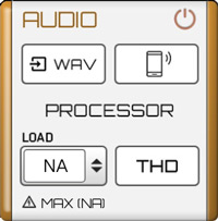
What You Can Do

2. Labels Tool

This tool is useful to perform the relative compression test. You can set any number of cylinder and their firing order and compute power.

3. 360-720° Tool

This tool allow to add the overlay of 720 degrees of crankshaft rotation in pressure waveforms. A middle cursor is moveable to allow relative measure of the angle. An option button allow to use different visualizations.

Audio Module

Note: this Module requires a specific license in addition to the basic HScope license.

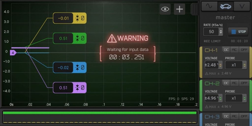
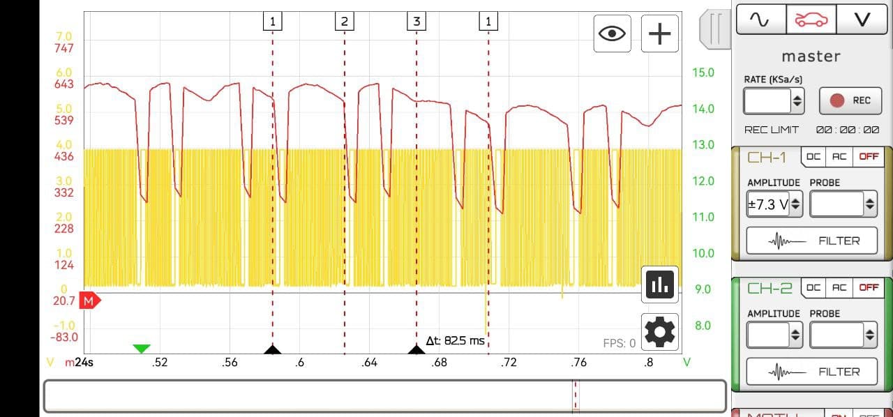
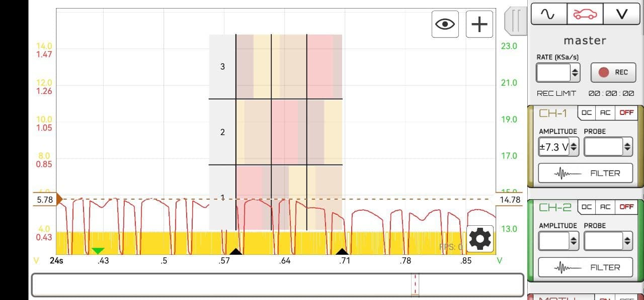
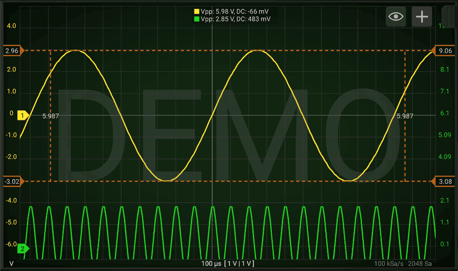
2. Hear the input signal from Channel-1 on phone

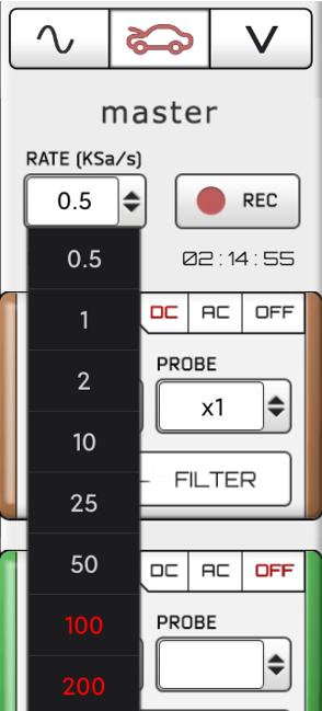
The oscilloscope signal can be sent to the phone speaker through real-time data streaming. While hearing the signal you can still navigate in the Oscilloscope graph or switch to the FFT graph. It works at sampling rates 25KSa/s and 50KSa/s. Since the oscilloscope can acquire low voltages this function is useful to check low signals in initial amplifier stages.

Note: this function is not supported by all the os

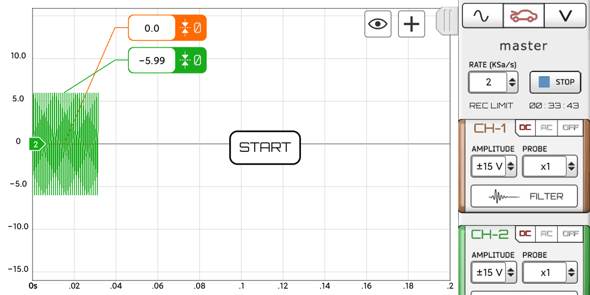
3. Compute the Output Power of an Audio Amplifier

The Audio Module can compute the output Power (RMS Power) of a Audio Amplifier by connecting the probe to the speaker connections and by selecting the impedance of the speaker in HScope. The maximum power is indicated in the Audio module panel and depends from the oscilloscope maximum input voltage. For increasing it, set a higher oscilloscope input voltage or use a x10 / x20 / x100 probe. The result is shown in real-time on the graph under the RMS value. For this measure you should input a sine wave in the amplifier. This signal could be produced by a portable MP3 player or by another phone App.

Pay attention: the sound generator cannot be the same phone running HScope since it cannot share the same GND of the oscilloscope.

Pay attention: the output of an audio amplifier could have high voltages. The GND of the probe should be connected to the GND of the amplifier or to the speaker wire connected to the GND. If both speaker wires are floating (neither one on GND), then the oscilloscope GND and phone box could be at a dangerous voltage. In this case you may look to some insulation solution like to use capacitors in series both to the probe tip and to the probe GND. (see EEVBLOG)

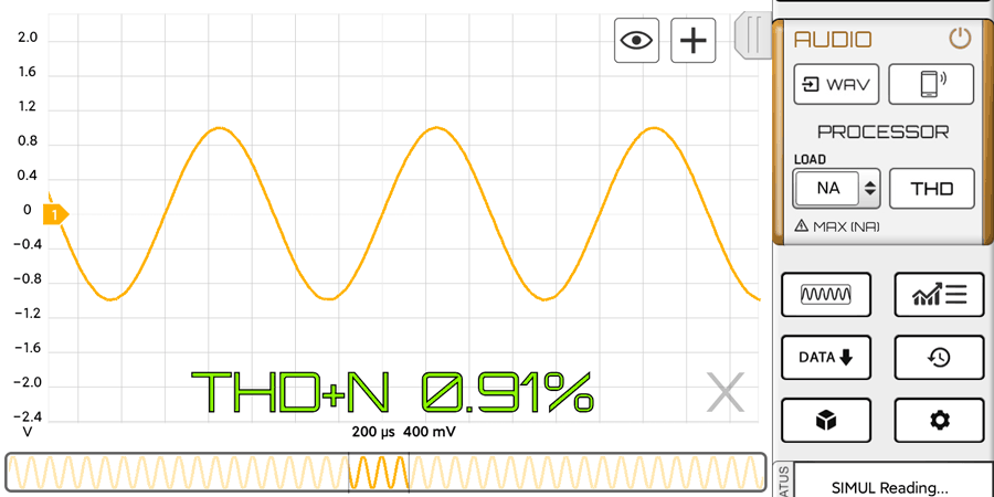
4. Compute the Audio Distortion (THD+N)

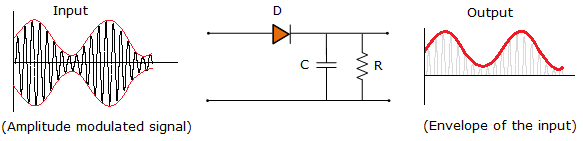
The primary job of any audio device is to faithfully reproduce or transmit the audio signal that is input to it. An ideal, linear audio device will produce an output signal that is an identical scaled version of its input signal. Anything that alters the input signal in any way, other than changing its magnitude, is known as distortion.

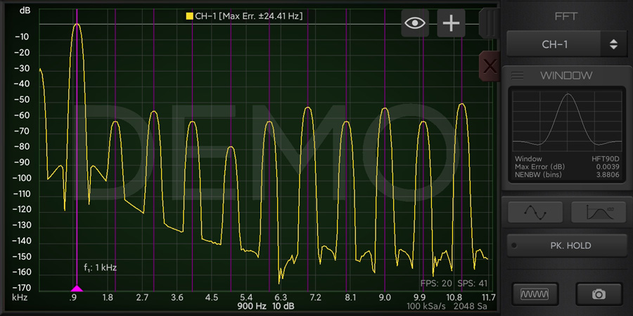
A classic means of detecting audio signal distortion is to stimulate a device under test (DUT) with a pure sine wave and then conduct a spectral analysis of the DUT output. Sine waves are used because a pure sine signal has the unique property that all its energy is concentrated at a single point in the frequency spectrum. This makes it easy to analyze the output from the DUT for unwanted distortion components. When a single sine wave is used as the stimulus, nonlinearities in the DUT cause harmonic distortion, wherein distortion components occur at harmonics (integer multiples of the sine signal’s frequency, or fundamental frequency).

Total Harmonic Distortion Plus Noise (THD+N)

The THD+N technique is the most common method of measuring harmonic distortion. In its basic form, it is implemented with a sharp notch filter tuned to the fundamental sine frequency, a bandwidth limiting filter, and an rms level meter. The notch filter removes the fundamental sine signal, leaving a residual signal which consists of the harmonics and noise. The THD+N Ratio is calculated as the bandwidth limited rms level of the residual divided by the rms level of the entire signal.

Samples for testing

If you want to test the THD processor you can import WAV files with known distortion. For example the file you can find at this link.

Resources

• Audio module demo on Youtube Playlist
• THD+N Calculator test on Youtube

PWM Module

This module is available just for few oscilloscopes as:

• Loto Oscilloscopes (OSC 482, OSC 802, OSC A02)
• Hantek 6022 (BE & BL)
• HS10X & H40X DIY Oscilloscopes
• HS502

It allow to use the output calibration pin (generally set to 1KHz square wave) to generate a PWM output signal. Max frequency and duty cycle range depends on the device (detail are in each oscilloscope page).

Example of usage as this video.

XY Plot

You can use this module only when the first 2 channels are active.
Channel-1 → plotted on X axis
Channel-2 → plotted on Y axis

Features

• Real-time processing
• Fading graphic effect
• Big graph space

On the left you can see 5 periods of both channel signals with the information about amplitude and frequency.

On the right there is the XY Plot with comparison information of the two signals. The phase shift is calculated with the Lissajous method and it is valid just for Sinusoidal Waveforms with same frequency.

Calculation of Time Delay

If you want to calculate the time delay for an arbitrary signal from 2 points of a circuit under analysis, just press the yellow/blue text and you will see this value obtained from the Cross-Correlation of the two signals.

Invert the Signals

If you want to invert one or both the signals, just Invert it in the Filter panel available for each channel.

Proof of Concept

The following video show the real-time capacity of this module.

Screenshots

Comparison test between HS-402 and Tektronix-465 oscilloscopes with PNP and NPN transistors.

FFT

Clicking on FFT button is possible to see the rapresentation of the signal in the Frequency Domain only for the first Channel. The range of visible frequencies on screen can be selecting zooming-in or out with the fingers on the screen.

Activating the STATS button is possible to see the top 3 frequencies in the selected frequencies range. These values are corresponding to the computed FFT values and not to the real values that can be checked better with the ruler.

FFT Windows

It is possible to select between standard windows and Flat Top windows for the FFT. Flat Top windows (HFT90D and HFT248D) are used when is required to determine the exact amplitude of a sinusoidal component in the input signal. They have bandwidths W_3dB of about 3 . . . 5 bins, roughly twice as wide as non-flat-top windows with comparable sidelobe suppression, but very low maximum amplitude error e_max.

WINDOWS SUMMARY

Bartlett	W3dB = 1.2736 bins emax = −1.8242 dB = −18.9430 %
Hanning	W3dB = 1.4382 bins emax = −1.4236 dB = −15.1174 %
HFT90D	W3dB = 3.8320 bins emax = −0.0039 dB = 0.0450 %
HFT248D	W3dB = 5.5567 bins emax = 0.0009 dB = 0.0104 %

Harmonic Cursor

When you use one single Vertical Cursor in the FFT module, it will show also the Harmonics of the selected frequency, up to the 10th harmonic.

Math Channel

To add a math channel, just click select MATH in the modules and you will see the Math configuration panel. You can quickly select one of the built-in functions, such as inversion or addition. All the standard arithmetic functions are supported along with more complex functions like demodulation and instant frequency of the signal.

With HScope currently you have available only 1 math channel.

List of functions

Basic functions:	– A (invert) A + B (sum) A – B (difference) A x B (multiply) A : B (divide)
Advanced functions:	demod (demodulation) freq (instant frequency)

Amplitude Demodulation

For some signals (for example from vibrations sensors), the information is carried by the amplitude (or envelope) of the signal. The demod() function allow to do this operation. Following is the equivalent circuit of this operation.

Instant Frequency

Visualize the instant frequency variation of the signal along time. The freq() function is useful for signal where frequency variation bring the useful information.

Sample application of this function to detect missfire with Automotive Module (detected 1 missfire event during long period recording):

Credits

• freq() function (or Instant Frequency) has been developed with the support of: Denis, Ravindra

Introduction – Oscilloscope Modules

Click on the “red cube” button to access the additional modules for the Oscilloscope.

1. Math Module: allow to compute Math operations among the first 2 channels.
2. FFT: allow to compute the FFT operation.
3. XY Plot: for comparing signals and compute phase shift.
4. Audio Module: for listening the input signal with the phone speaker and compute Amplifiers Power. Instructions here.
5. Digital Module: for analize digital signals.
6. PWM Module: if available in the oscilloscope hardware it control the PWM output.

Tools

Click on the “eye” icon to open the View Tools.

1. Zoom the waveforms to fit the screen vertically.
2. Align the waveforms on the same Zero Level.
3. Align the waveform vertically keeping spacing among them.
4. Scale the second channel signal to fit the first channel signal (so to compare the shape).

Press the “+” icon to activate the Supporting Tools.

1. Vertical Cursors: it show vertical cursor.
2. Horizontal Cursors: it create one horizontal cursor.
3. Annotation Tool: you can write labels on the graph and position them on the desired location.

Additional tools may be present according the additional modules installed (ie. Automotive Tools in the picture).

1. Vertical Cursors

Activating one vertical cursor allows you to measure amplitude of the signals at a certain point. By pressing 2 fingers on the bottom part of the graph you can enable 2 cursors and have relative measurements. (as time and frequency associated to the selected period).

For removing the cursors just push them out of the screen (to the left or to the right), on the red area.

HScope allows a maximum of 2 Vertical Cursors.

2. Horizontal Cursors

You can enable one or more Horizontal cursors. When you have 2 Horizontal cursors on the screen, you can see also the distance between the 2 cursors.

Horizontal cursors works as the Vertical ones.

3. Annotation Tool

When you create a new Annotation you can set the text. Later you can change the location of the annotation but not its text. You can select an Annotation by clicking on it.

To delete an Annotation just move it behind the red bar.