Tools

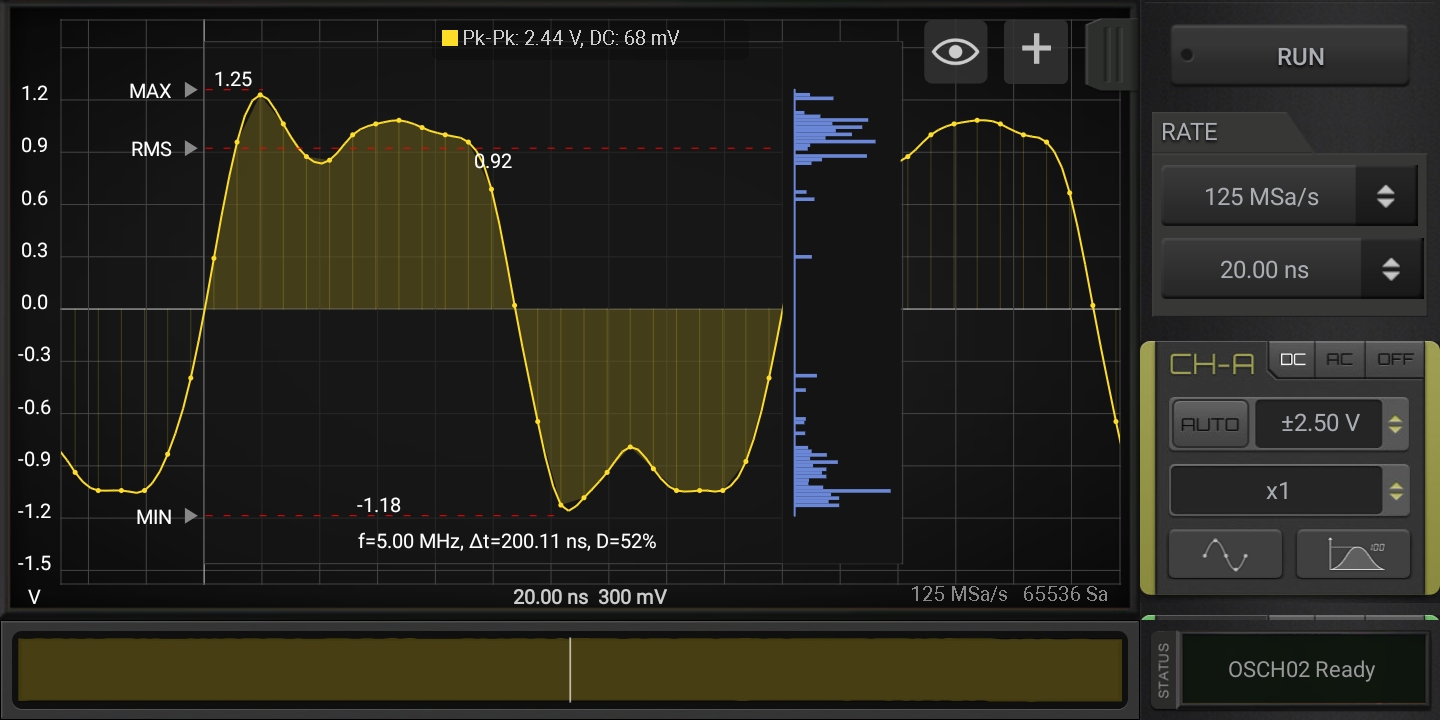
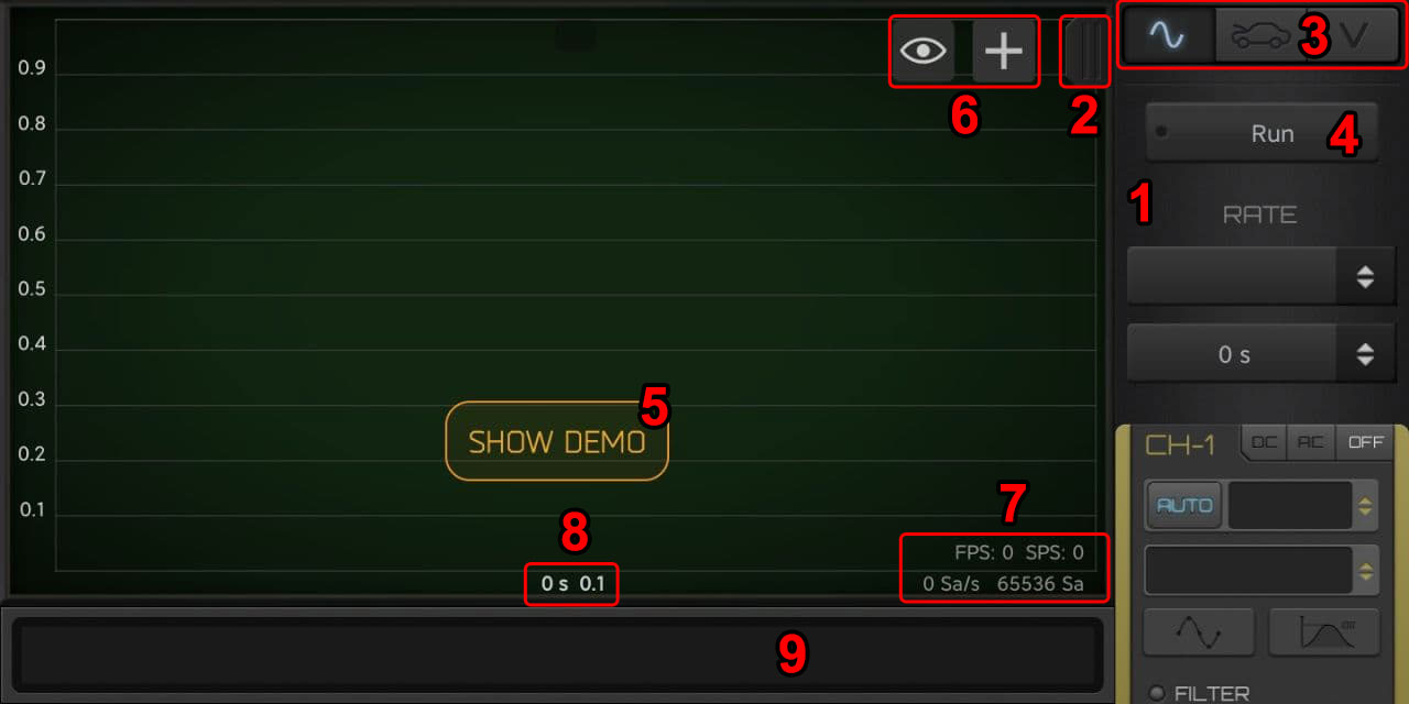
Click on the “eye” icon to open the View Tools.

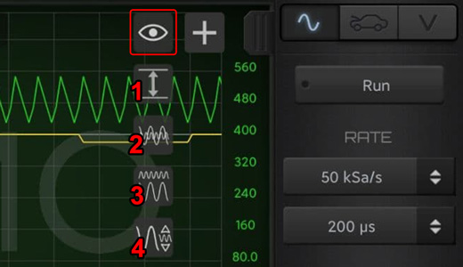
1. Zoom the waveforms to fit the screen vertically.
2. Align the waveforms on the same Zero Level.
3. Align the waveform vertically keeping spacing among them.
4. Scale the second channel signal to fit the first channel signal (so to compare the shape).

Press the “+” icon to activate the Supporting Tools.

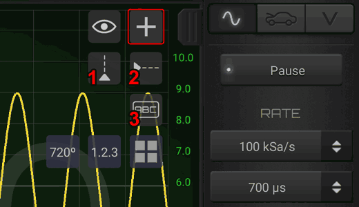
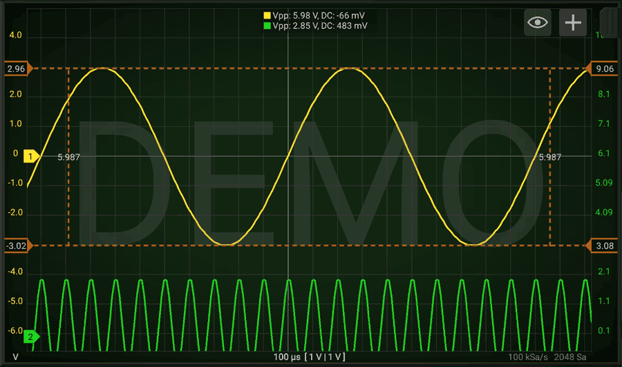
1. Vertical Cursors: it show vertical cursor.
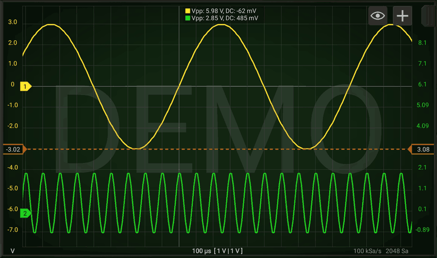
2. Horizontal Cursors: it create one horizontal cursor.
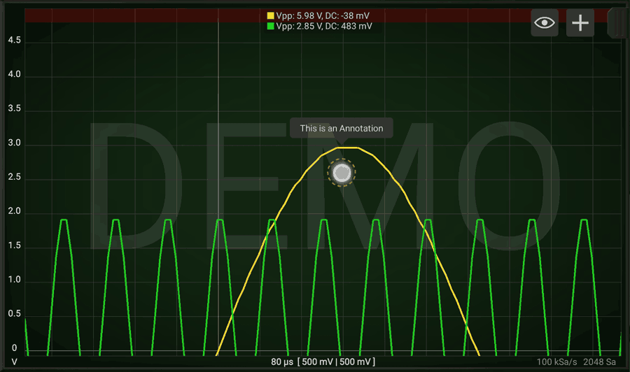
3. Annotation Tool: you can write labels on the graph and position them on the desired location.

Additional tools may be present according the additional modules installed (ie. Automotive Tools in the picture).

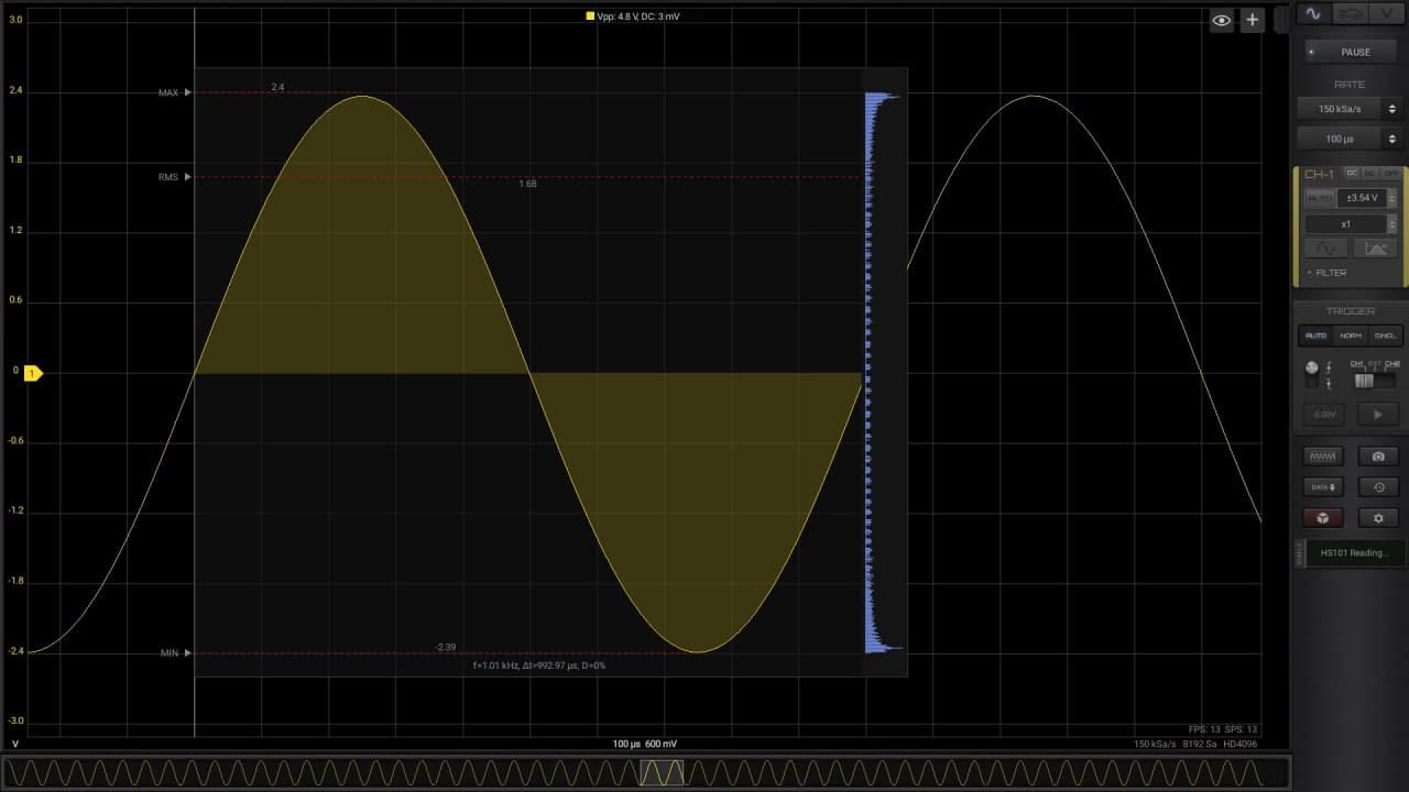
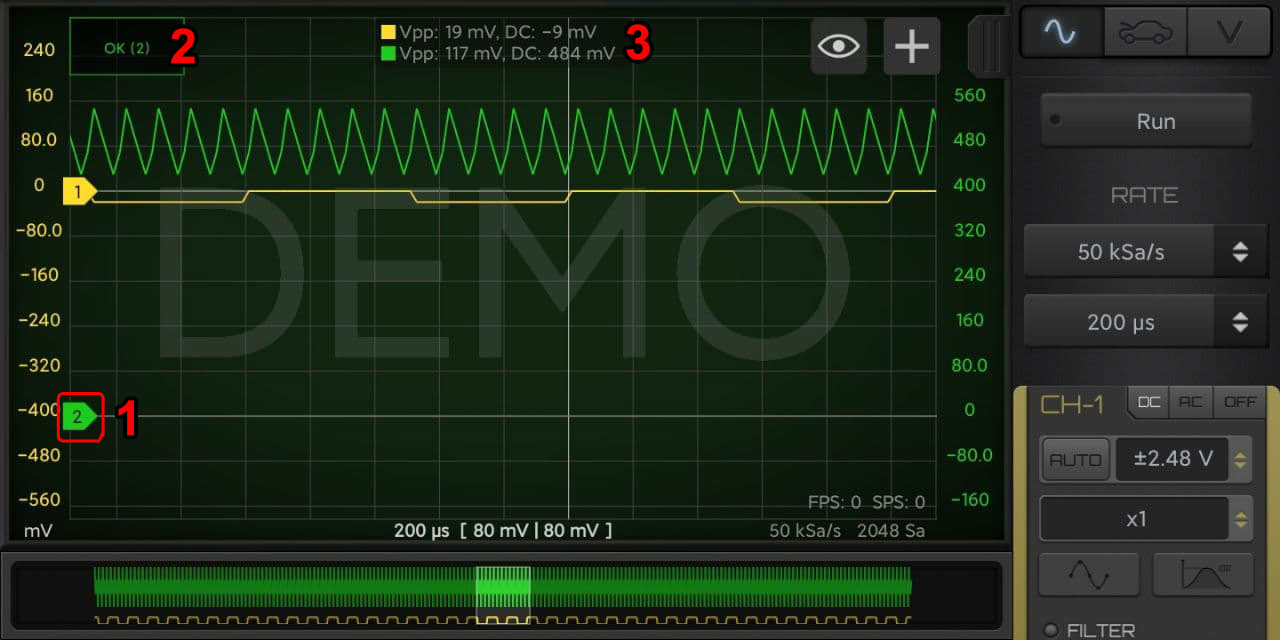
1. Vertical Cursors

Activating one vertical cursor allows you to measure amplitude of the signals at a certain point. By pressing 2 fingers on the bottom part of the graph you can enable 2 cursors and have relative measurements. (as time and frequency associated to the selected period).

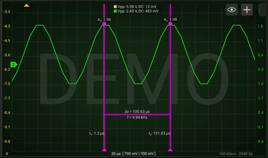
For removing the cursors just push them out of the screen (to the left or to the right), on the red area.

HScope allows a maximum of 2 Vertical Cursors.

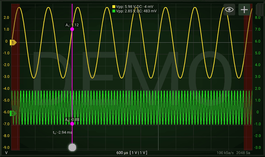
2. Horizontal Cursors

You can enable one or more Horizontal cursors. When you have 2 Horizontal cursors on the screen, you can see also the distance between the 2 cursors.

Horizontal cursors works as the Vertical ones.

3. Annotation Tool

When you create a new Annotation you can set the text. Later you can change the location of the annotation but not its text. You can select an Annotation by clicking on it.

To delete an Annotation just move it behind the red bar.

Setting the Trigger

The Trigger allow you to see the signal stable on the screen since the Trigger set what is the starting point for drawing the signal. Even if the input signal can be periodic in some way, on each scan its position can be found translated since the acquisition time is random and it cannot be synchronous with the period of the input signal.
The starting point for a signal can be identified with:

• a Voltage Level (Trigger Level);
• a tendency (or Slope) which means if the signal is passing the Voltage Level going up or down.

Once decided the kind of trigger (AUTO, NORMAL, SINGLE), you can set the SLOPE (arrow up or down) and the input Channel (only CH1 and CH2 are working and they are oscilloscope depending).

• AUTO Trigger: set the Trigger Level as the middle level of the input voltage.
• NORMAL Trigger: allow you to set the Voltage Level for the trigger. Every time the condition is met the signal is visualized on the screen.
• SINGLE Trigger: as Normal Trigger but will show the signal just at the first occurrence of the condition, then it stops the acquisition. You can resume the acquisition by pressing the play button.

Filters

You can apply filters to each channel (button FILTER). Filtering operation may change the original signal in reversible or irreversible way. Irreversible filtering means that the operation modify the original signal in a way that later the original signal cannot be restored.

Type of Filtering	Description	Reversible
Invert (inversion)	It invert the input signal (the signal will be mirrored respect the 0 level)	Yes
Low Pass	The frequencies over the defined frequency will be attenuated.	No*
High Pass	The frequencies below the defined frequency will be attenuated.	No*

* In Automotive Module the filtering can be reversible until the waveform is not saved. After saving the filtered data will be saved and there is no way to reverse to the original waveform or change the filtering parameters.

Filters Response in Frequency

You can set the cutoff frequency of the filter. In case of low-pass and high-pass filter you just set the one frequency, while in case of band-pass and band-stop filters you must set 2 frequecies, one of start and one of end. At the cutoff frequency the signal is attenuated of 70.7% of its amplitude and keep to be attenuated more an more according the graph above.

For example if you set a low-pass filter at 100Hz it means that you will see all the components of the signal up to around 100Hz. After 100Hz they will be progressively attenuated.

The inclination of the attenuation curve depends from the filter order. Higher is the order and more rapids is the curve.

A typical usage of a low-pass filter is to filter out the noise from the signal of interest, a way to “clean” the waveform. Here an example of signal cleaning with a low-pass filter:

Setting the Channels

Differently from other oscilloscopes, in HScope you can set the voltage input range for each channel. The concept of Volts/division is just reported as information but it is not really practical since the signal can be zoomed and shifted on the screen and measured with absolute scales and relative cursors.

1. DC/AC/OFF Button: can switch the input coupling mode to DC, AC or switch off the channel.
2. Input Voltage Selector: it set the oscilloscope maximum input range.
3. AUTO Button: automatically switch the input voltage according the input signal.
4. Probe Selector: set the current hardware probe used by the oscilloscope on the channel.
5. Samples Button: by enabling it you can see the actual samples by zooming in the signal on the screen.
6. Statistics Button: it show the main statistics for periodic signals by showing the details of 1 period of the main frequency. HScope support 2 kind of statistics, press 1 time for the simple one, press another time for the Histogram, a last time to turn them off.
7. Filters: to enable filters on the channel (check the Filters section).
8. Channel Name: you can change the channel name by clicking here. The new name will be shown on the report and saved in the waveform file.

1. DC/AC/OFF Button

Selecting DC the signal goes to screen AS-IS (with AC and DC components), selecting AC the signal pass into a filter (that can be hardware or software according the device) so that on screen and in computation is considered just the AC component.

2. Input Voltage Selector

This value is oscilloscope depending and change according the actual calibration. To benefit of the highest vertical resolution it is suggested to use the lowest range which include the measured signal.

3. AUTO Button

Selecting the button AUTO the software automatically set the input voltage selector according to the signal. It is intended to be use only for time invariant signals (like a sine wave) otherwise the input range will be changed very time the input signal change. This function is limited just to high voltage ranges. Lower voltage selection should still come manually.

4. Probes Selector

This setting won’t affect the hardware settings but it will affect the final readings since the data will be computed according the probe settings.

IMPORTANT: Probe setting MUST reflect the probe hardware to avoid damage to the device or wrong readings. (ie: you can set x10 in HScope only if the hardware probe has x10 switch selected)

In case you need to measure stronger signals the Probe should have a switch that allow to attenuate the input signal. If you change the switch of your probe to the position x10, the input signal will be attenuated by a factor 10. This means that using the Oscilloscope range ±5V with a probe x10 you can see signals up to ±50V (50V / 10 = 5V). In visualization the App already calculate this scaling factor, so if you use a probe x10 just select in the Channel configurations the factor x10 and play with the voltage ranges (it will show you the possible range you can select).

On the market are available different kind of probes (also associated to different units like Ampere,…). You can add or download new probes in the Settings → Probes panel.

VOLTAGE RANGES (SAMPLE)

• Native Hardware Input Ranges
  (with Probe x1) ±0.5V, ±1V, ±2.5V, ±5V
• Input Ranges after using Probe
  (with Probe x10) ±5V, ±10V, ±25V, ±50V

6. Statistics

• First press: full statistics
• Second press: histogram
• Third press: statistics off

Setting the Rate

Differently for standard oscilloscopes, in HScope you can select the acquisition rate of the oscilloscope. Selecting the rate means to set how many points/second (or Samples/s) you want to use to scan the input signal. After selecting the rate you can choose the time/division.

This value is also related to the maximum frequency you suppose to find for your signal. Assuming your signal is a Sine like shape you may practically need at least 10 points inside one period.

So with a rate of 100 KS/s (Kilo Samples / second) you can see well waves till 10KHz. If these waves have faster variations then you need to increase the rate level.

Square signals has infinite bandwidth, so they may requires high sampling rates to see well the edges.

ROLL MODE RATES

Roll mode rates are slow rates indicated in blue color in the rate list selector. At these rates the signal update in real time on the main screen going from left to right.

Currently is is not possible to use Trigger functions with a Roll Mode rate.

Waveforms Management

With HScope you can import/export and share waveforms.

Most of the operations are done in the Waveform Manager:

1. Import from Cloud button: import a Waveform from the Cloud (it requires to know the Waveform ID, see under)
2. Import Waveform file from Phone (HScope .zip file format)
3. Import all Waveforms from a folder in the Phone (HScope .zip file format)

You can see additional information about the waveform by pressing the Show Details button:

Waveform File Format

The Waveforms are saved inside .zip files. The package contain waveform information and data in an open XML format, and the pictures/photos related to the waveform.

You can also export the waveform in another format by using the Share Button.

Cloud Sharing

You can send waveforms to colleagues or friends by using the Cloud Sharing, a free feature in HScope.

Click on the Share Button, then you select the Share via Cloud button:

On the other side, use the Import from Cloud button to input the number of the Waveform you want to import.

Note: If you copy to the Clipboard the Waveform ID from a chat, or a sentence containing it, when you press Import from Cloud button it will recognize automatically the number from the Clipboard.

The Main Interface

1. Main menu: you can scroll to access all controls.
2. Hide/Show menu button.
3. Mode Switch button: it switch among the main interfaces – Oscilloscope, Automotive (it requires the specific module) and Data Logger.
4. Run/Stop button: start and stop the acquisition (when the oscilloscope is connected).
5. DEMO button: start the Demo mode with a sample signal so to try the app and the functions.
6. Tools buttons (see the specific guide)
7. Statistics: show the current sampling rate and the number of samples acquired in each scan. When enabled in the settings you can see the FPS/SPS value. SPS: Scan Per Second: the number of data buffers acquired from the oscilloscope each second. FPS: Frame Per Second: the number of graphic frames showed on screen each second.
8. Time/div, Volt/div: it show the X and Y quantity for each division.
9. Data Scroller: show the whole data buffer and allow you to fast scroll the data.

Finger operations

Scroll

Use one finger on the screen to scroll the signal in all directions.

Zoom

Use 2 fingers to zoom the signal in or out. The is no limit for zoom in. Zoom out is limited to the max area used by the signal.

Auto Zoom

Tap 2 times on the screen to get the signal zoom to fit the screen.

Adjust Signals Position / Scale

When running you can see the channel signals in different colors.

1. Each channel position can be moved by clicking on the handler on the left. While moving a channel you can also zoom it, changing its scale respect the other channels.
2. Confirm the channel position and scale by clicking on this button or wait 3 seconds for auto-confirm.
3. Channels basic stats: amplitude peak-to-peak and DC value (when the channel input is set on DC coupling mode).

Migrate to Android 10+

Read this part if you want to migrate your old HScope data on a new Android 10+ device.

Introduction

In Android 10+ if you want HScope to save and open waveforms, you should authorize the app to access a specific user folder. For performances reasons HScope will keep all data in its private folder and synchronize this data with the public user folder in order to avoid data loss and to allow the user to save or share this data.

The data in the public user folder (ie. /Documents/HScope) should not be modified manually otherwise you need to delete the app data (in the Android settings) and do this procedure again to keep the data syncronized.

1. Copy the data

Copy all HScope data on the new Android device. Source is /Downloads/HScope, destination can be under the Documents or Downloads folder (ie. /Documents/HScope).

2. Configure the Documents Folder in HScope

In Settings → System select the folder where you copied the HScope data (public Documents Folder).

After you select the HScope folder the app will import all the waveforms.

3. Import the Probe Settings

In Settings → Probes go in the download panel, then click on the folder icon (on top-right).

Select the file Probes.cfg in HScope documents folder. This operation will import all the previous probes settings.

4. Import other Waveforms (optional)

In the Waveforms screen (both Oscilloscope and Automotive mode) click on the folder icon (on top-right).

Select the folder of the Waveforms that you want to import (ie. /Scope or /Automotive under /Documents/HScope/). All the waveforms in the selected folder will be imported inside the Oscilloscope or Automotive list.

In case you import the wrong folder in the wrong HScope section (for example Automotive files inside the Oscilloscope list), you can delete all the app data in the Android Application Settings and do the importing again.

Warning: after you import the waveforms data, the data will the linked so if you delete a waveform in HScope, the waveform will be deleted also in the public Documents Folder. Also for the probes, any change to the list will overwrite the Probes.cfg file in the public Documents Folder.

First Connection

After installing the App, connect the USB Oscilloscope with an OTG cable. The App should detect automatically the Oscilloscope and ask the Authorization to use the USB Port. This Authorization may be asked twice and you can select the box “remember the choice” if you don’t want this window show again at the next connection.

If the everything works correctly you should see the signal on the App screen.

WiFi Devices

For WiFi devices (like Hantek iDSO1070 and the DIY HS402 WiFi) first connect the phone to the oscilloscope WiFi network, then open the App. The App should connect to the Wifi oscilloscope automatically (pay attention to enable the WiFi connection in the Settings).

Sample System

Setup used for the System testing (Oscilloscope not in the photo):