This module is available just for few oscilloscopes as:
Loto Oscilloscopes (OSC 482, OSC 802, OSC A02)
Hantek 6022 (BE & BL)
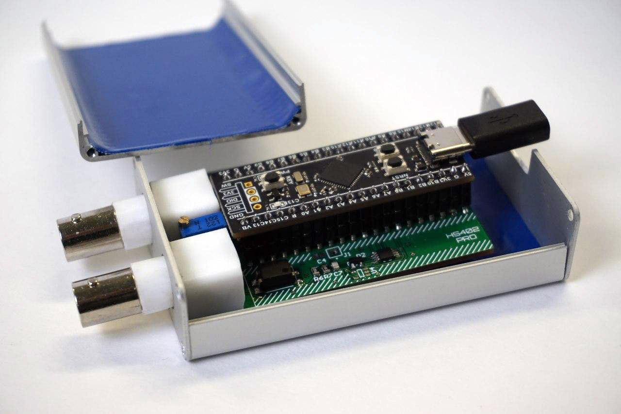
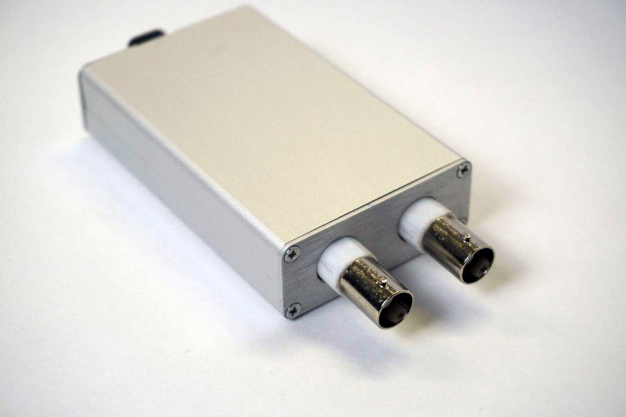
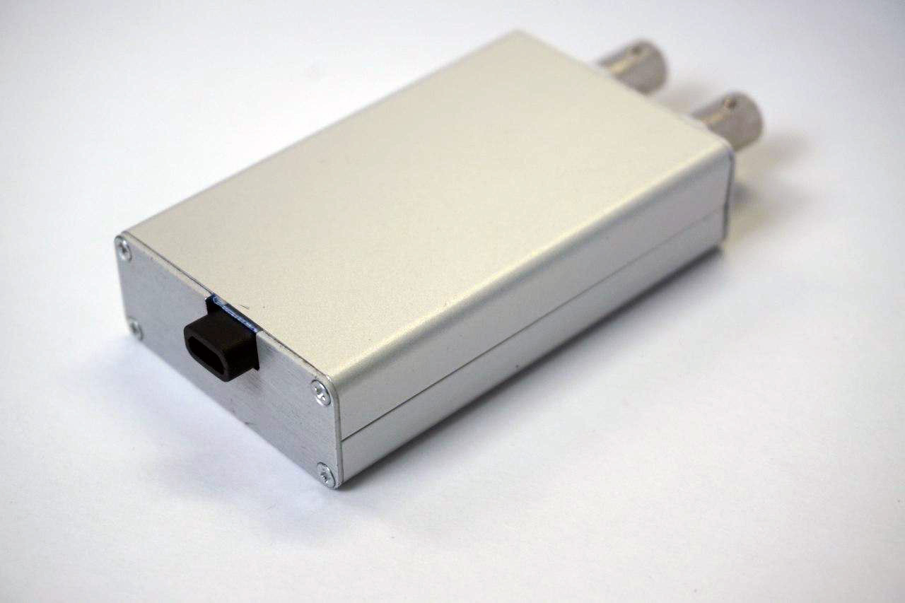
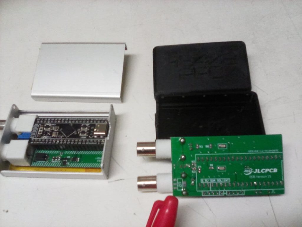
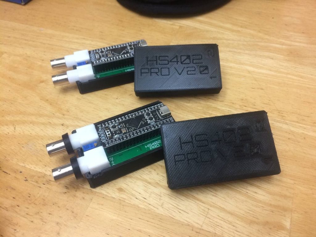
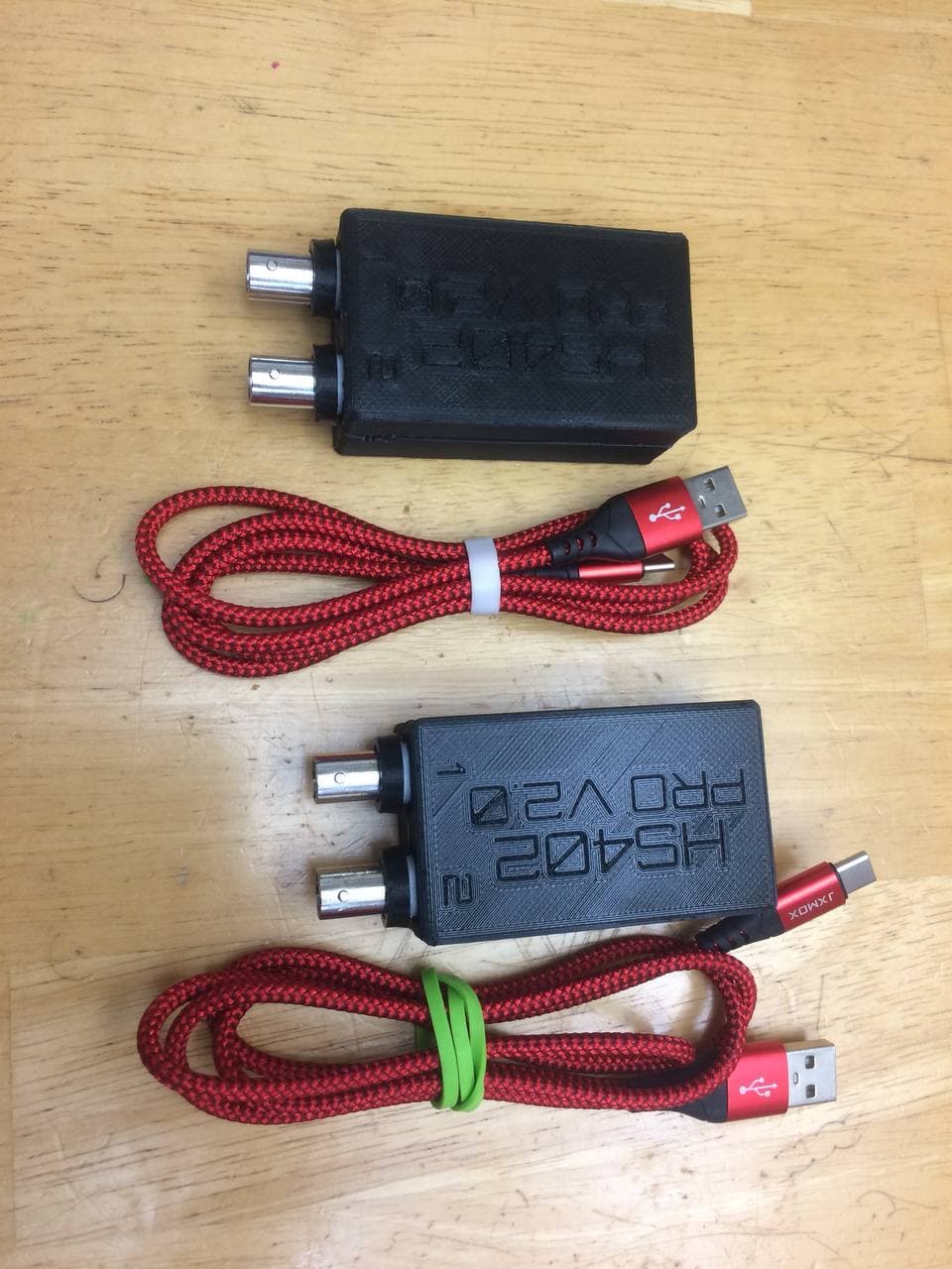
HS10X & H40X DIY Oscilloscopes
HS502
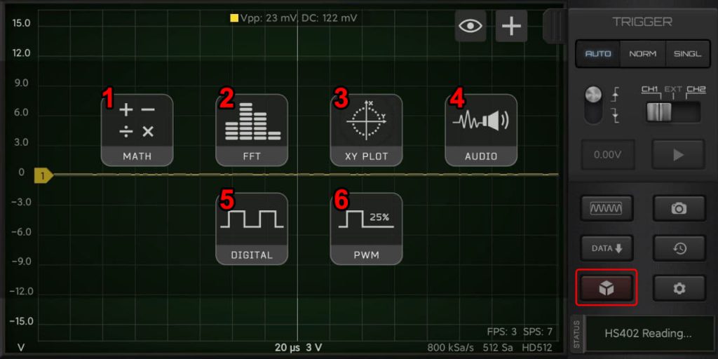
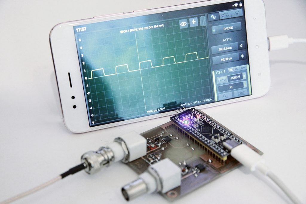
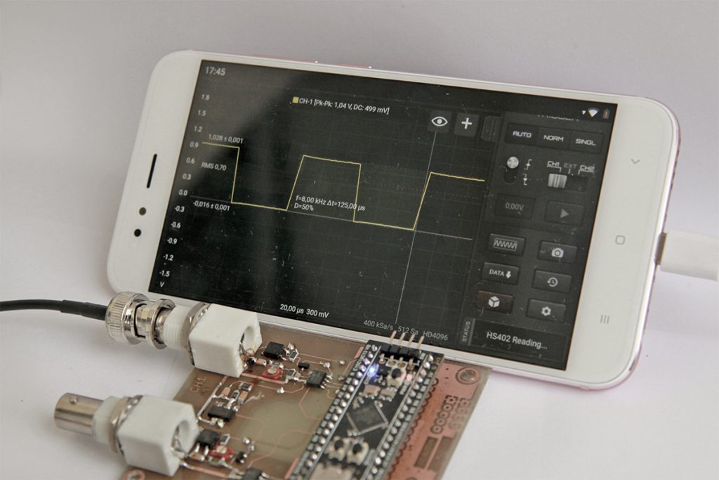
It allow to use the output calibration pin (generally set to 1KHz square wave) to generate a PWM output signal. Max frequency and duty cycle range depends on the device (detail are in each oscilloscope page).
You can use this module only when the first 2 channels are active. Channel-1 → plotted on X axis Channel-2 → plotted on Y axis
Features
Real-time processing
Fading graphic effect
Big graph space
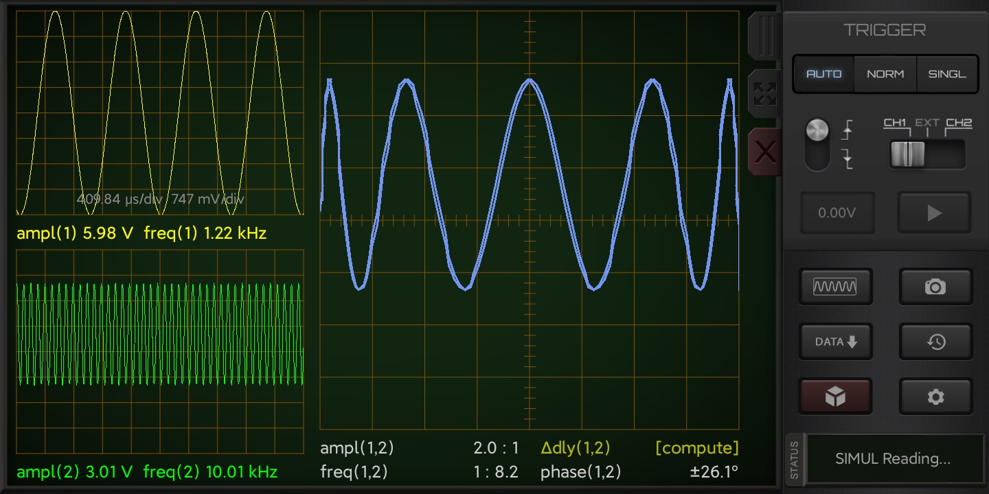
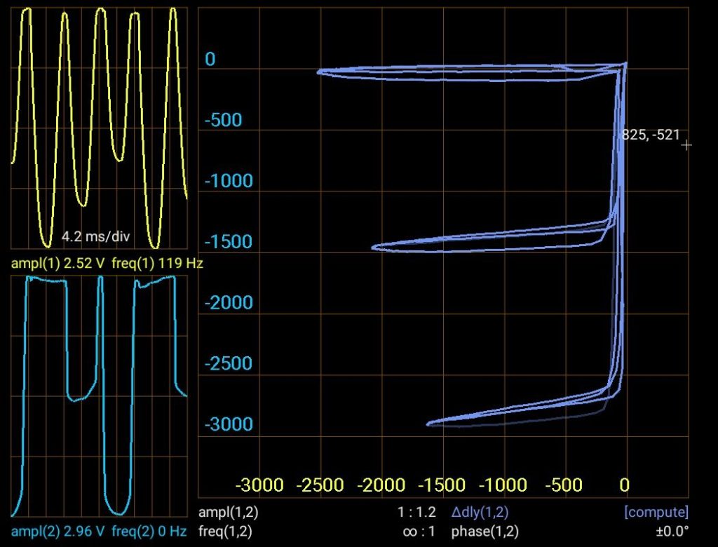
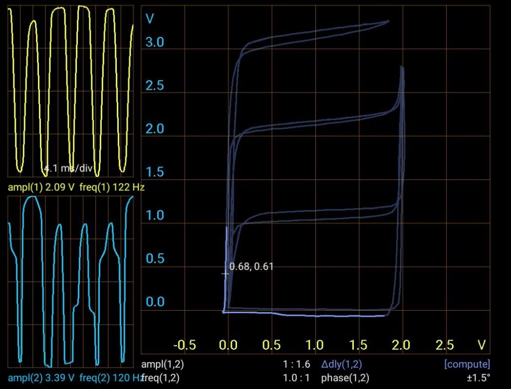
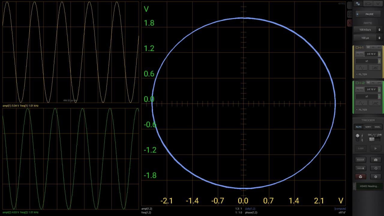
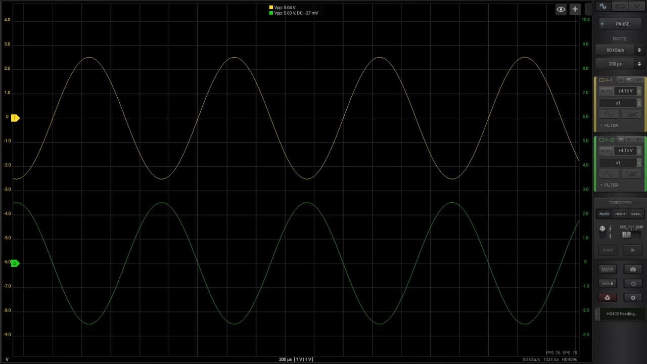
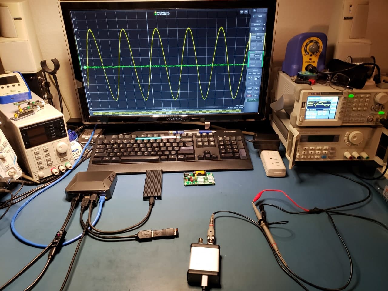
On the left you can see 5 periods of both channel signals with the information about amplitude and frequency.
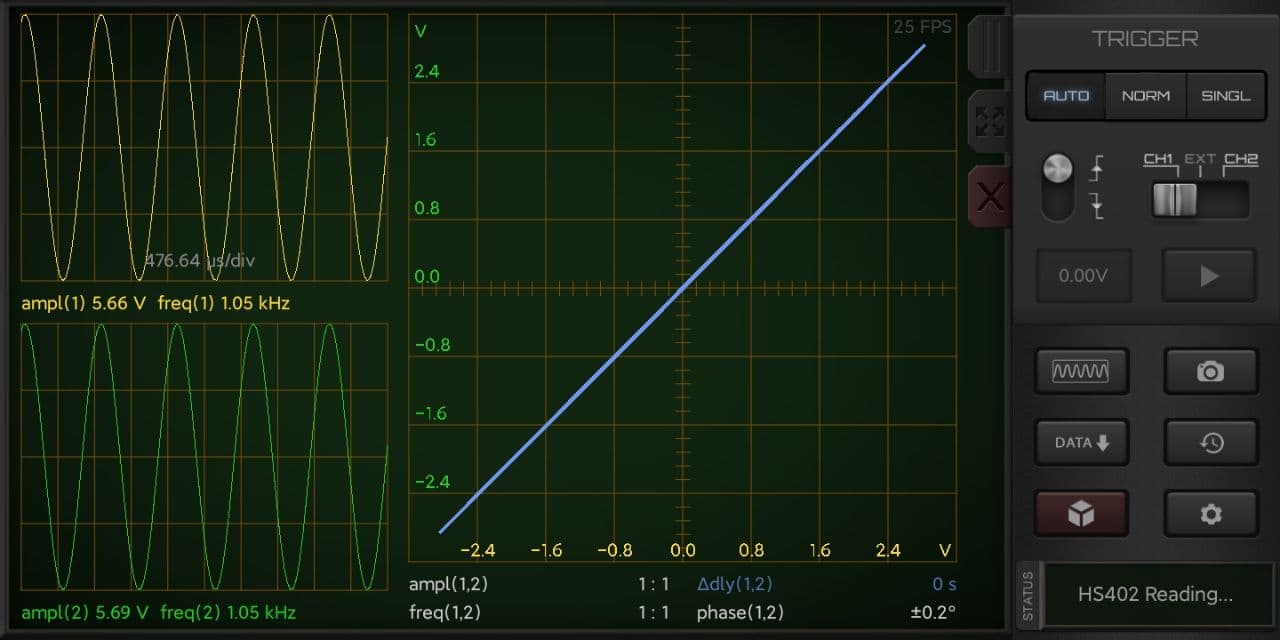
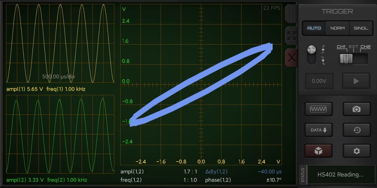
On the right there is the XY Plot with comparison information of the two signals. The phase shift is calculated with the Lissajous method and it is valid just for Sinusoidal Waveforms with same frequency.
Calculation of Time Delay
If you want to calculate the time delay for an arbitrary signal from 2 points of a circuit under analysis, just press the yellow/blue text and you will see this value obtained from the Cross-Correlation of the two signals.
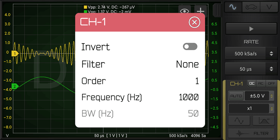
Invert the Signals
If you want to invert one or both the signals, just Invert it in the Filter panel available for each channel.
Proof of Concept
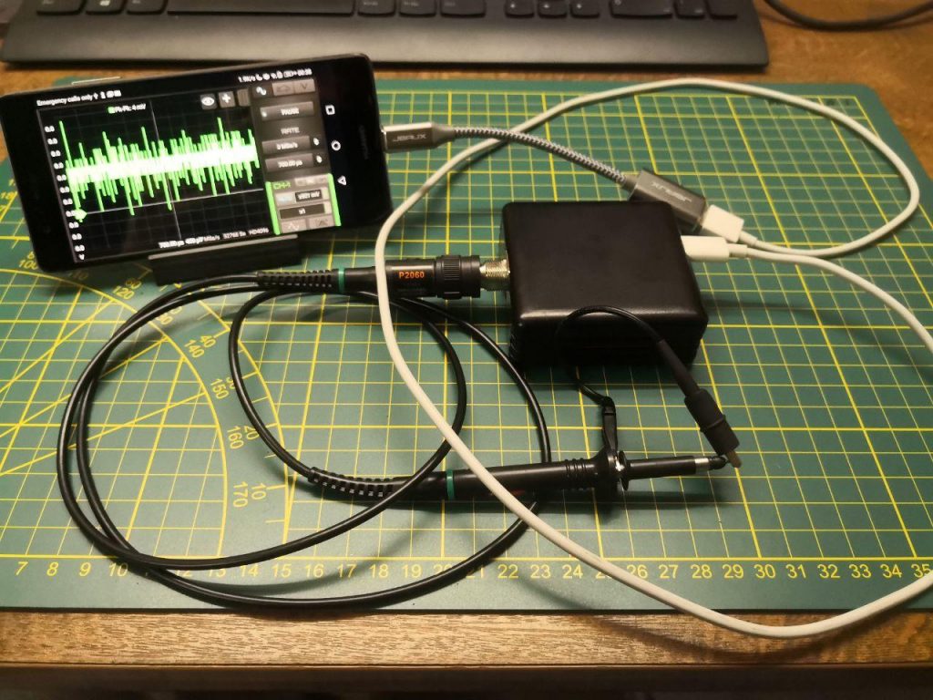
The following video show the real-time capacity of this module.
Screenshots
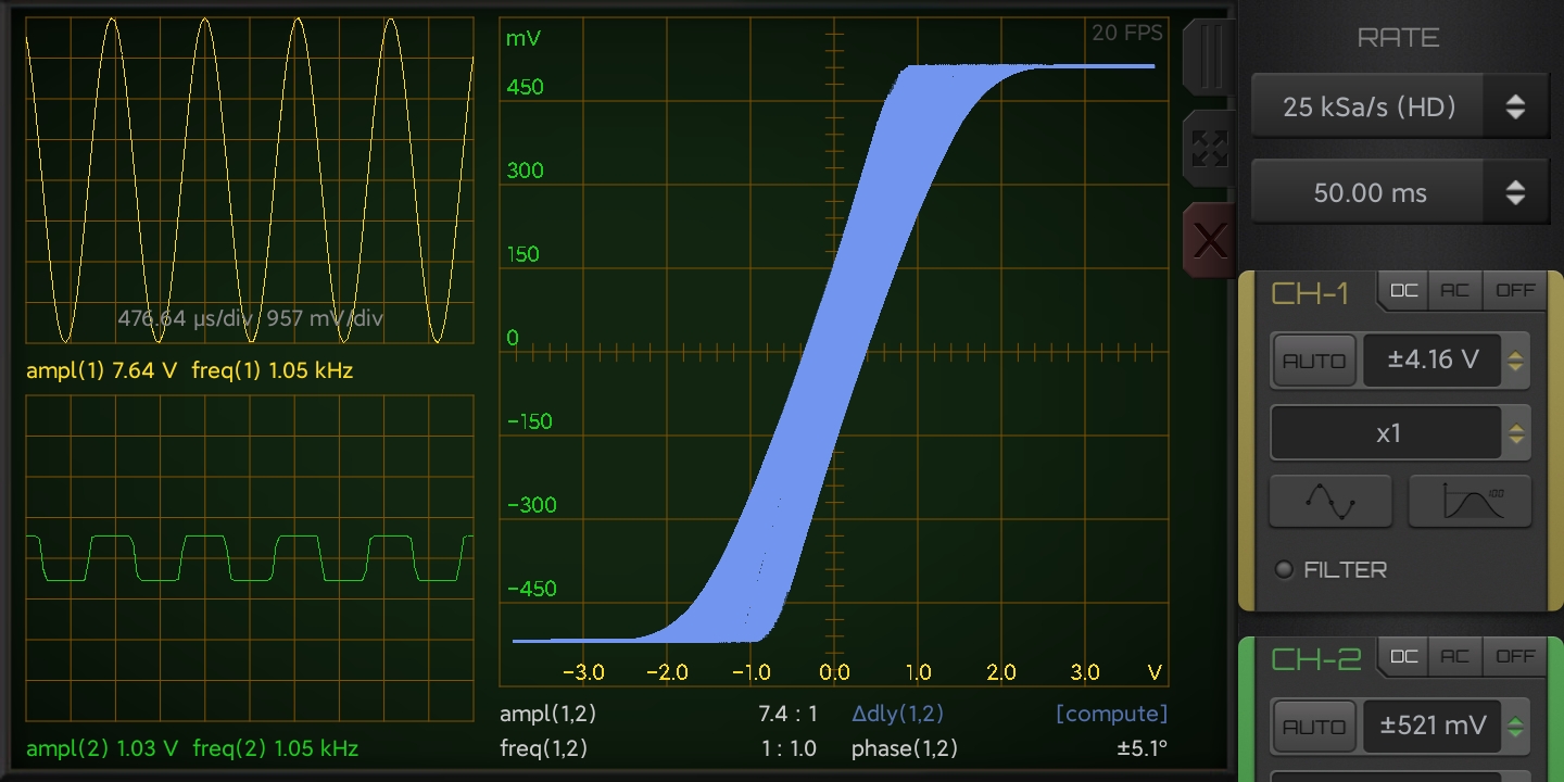
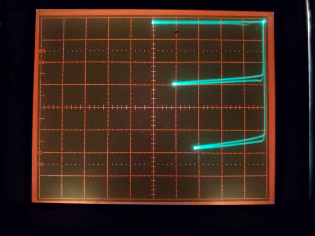
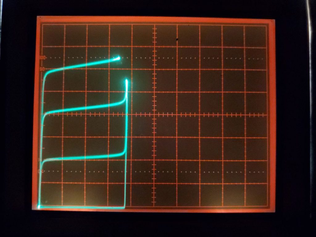
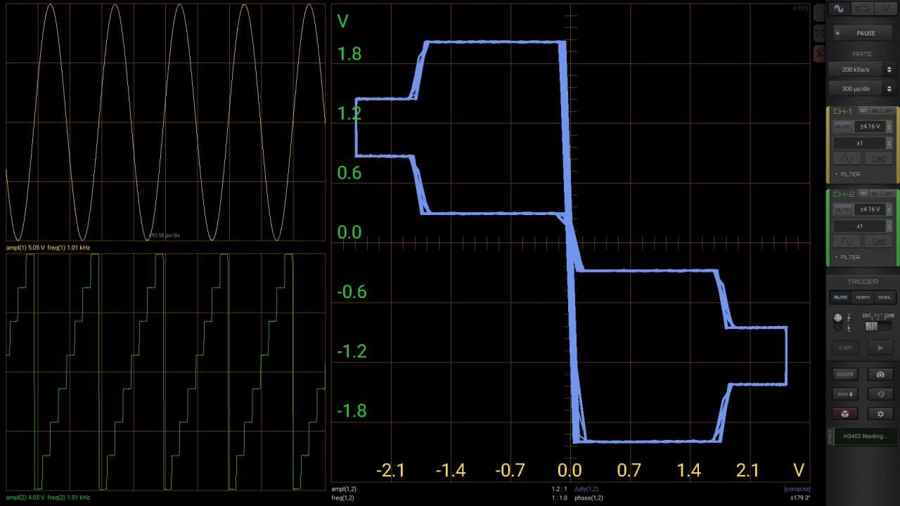
Comparison test between HS-402 and Tektronix-465 oscilloscopes with PNP and NPN transistors.
Images of courtesy from @Jim in @HScope Telegram group
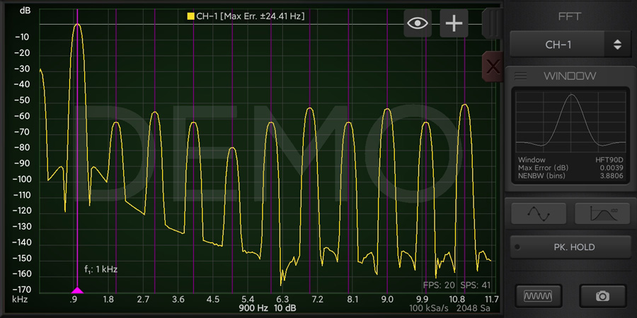
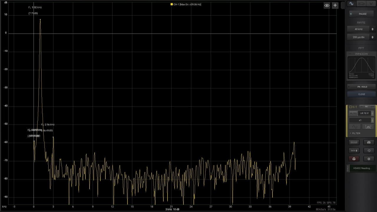
Clicking on FFT button is possible to see the rapresentation of the signal in the Frequency Domain only for the first Channel. The range of visible frequencies on screen can be selecting zooming-in or out with the fingers on the screen.
Activating the STATS button is possible to see the top 3 frequencies in the selected frequencies range. These values are corresponding to the computed FFT values and not to the real values that can be checked better with the ruler.
FFT Windows
It is possible to select between standard windows and Flat Top windows for the FFT. Flat Top windows (HFT90D and HFT248D) are used when is required to determine the exact amplitude of a sinusoidal component in the input signal. They have bandwidths W3dB of about 3 . . . 5 bins, roughly twice as wide as non-flat-top windows with comparable sidelobe suppression, but very low maximum amplitude error emax.
WINDOWS SUMMARY
Bartlett
W3dB = 1.2736 bins emax = −1.8242 dB = −18.9430 %
Hanning
W3dB = 1.4382 bins emax = −1.4236 dB = −15.1174 %
HFT90D
W3dB = 3.8320 bins emax = −0.0039 dB = 0.0450 %
HFT248D
W3dB = 5.5567 bins emax = 0.0009 dB = 0.0104 %
Sample FFT Windows
Harmonic Cursor
When you use one single Vertical Cursor in the FFT module, it will show also the Harmonics of the selected frequency, up to the 10th harmonic.
To add a math channel, just click select MATH in the modules and you will see the Math configuration panel. You can quickly select one of the built-in functions, such as inversion or addition. All the standard arithmetic functions are supported along with more complex functions like demodulation and instant frequency of the signal.
With HScope currently you have available only 1 math channel.
List of functions
Basic functions:
– A (invert) A + B (sum) A – B (difference) A x B (multiply) A : B (divide)
Advanced functions:
demod (demodulation) freq (instant frequency)
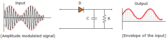
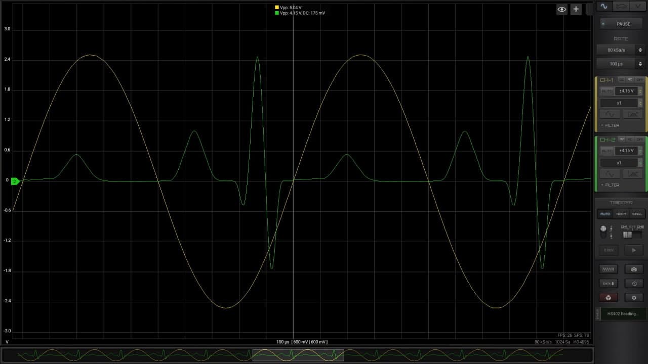
Amplitude Demodulation
For some signals (for example from vibrations sensors), the information is carried by the amplitude (or envelope) of the signal. The demod() function allow to do this operation. Following is the equivalent circuit of this operation.
Envelope Detector
Instant Frequency
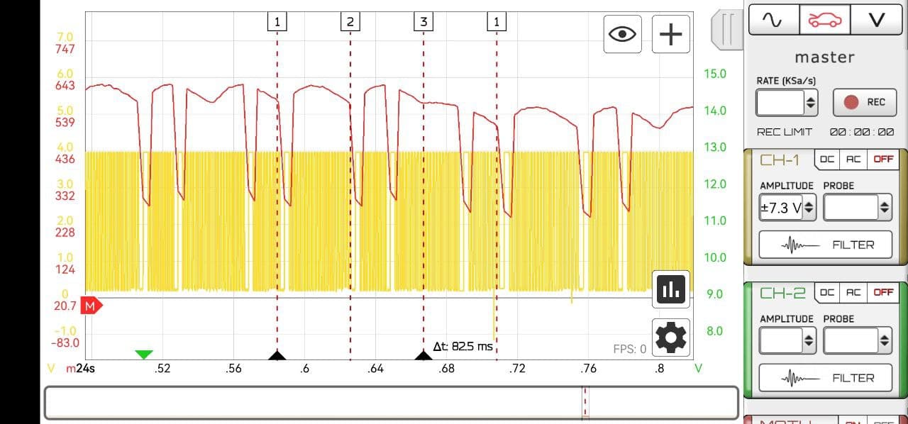
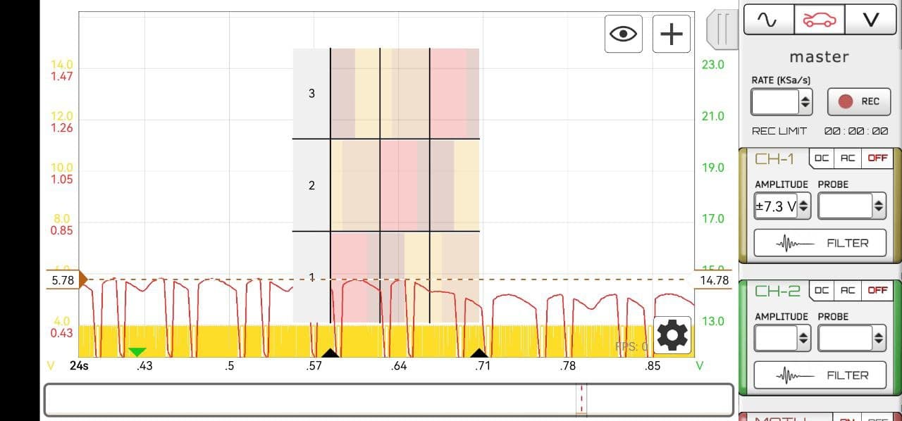
Visualize the instant frequency variation of the signal along time. The freq() function is useful for signal where frequency variation bring the useful information.
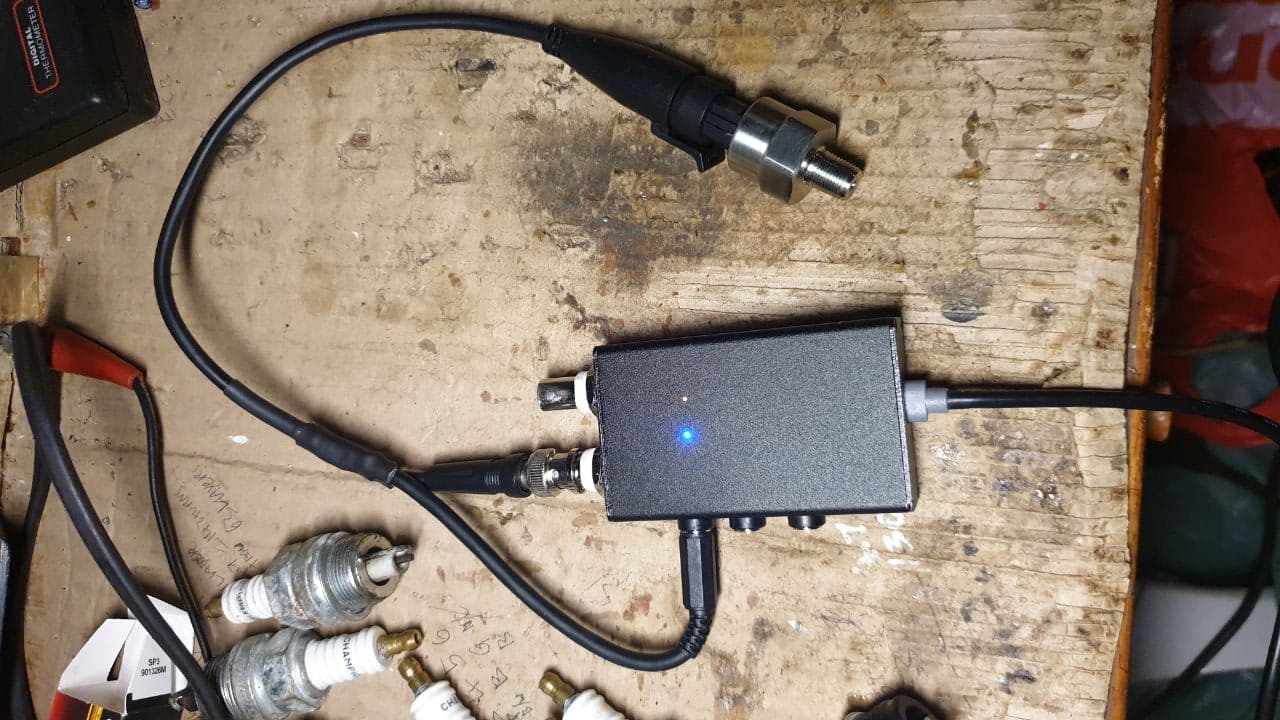
Sample application of this function to detect missfire with Automotive Module (detected 1 missfire event during long period recording):
Credits
freq() function (or Instant Frequency) has been developed with the support of: Denis, Ravindra
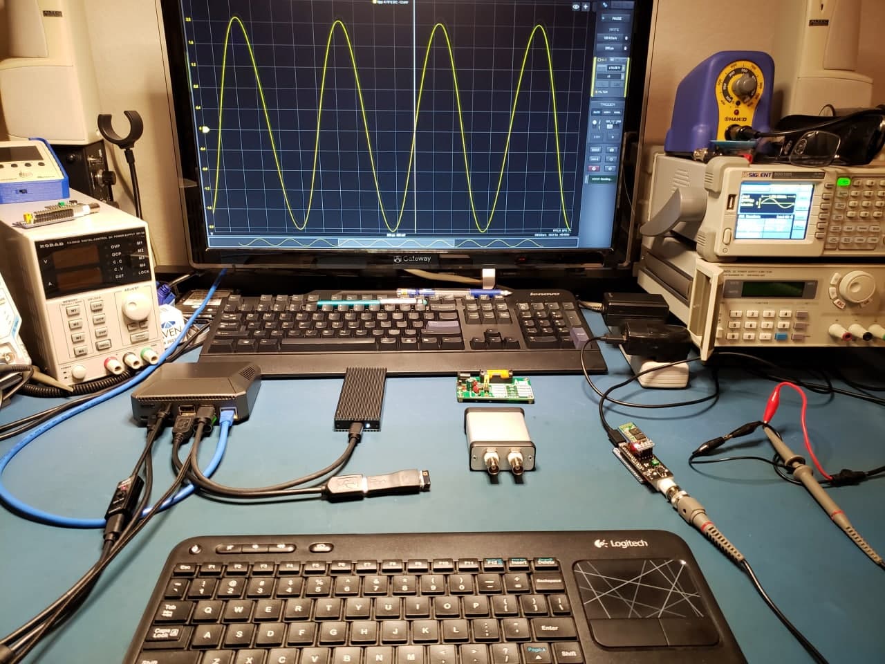
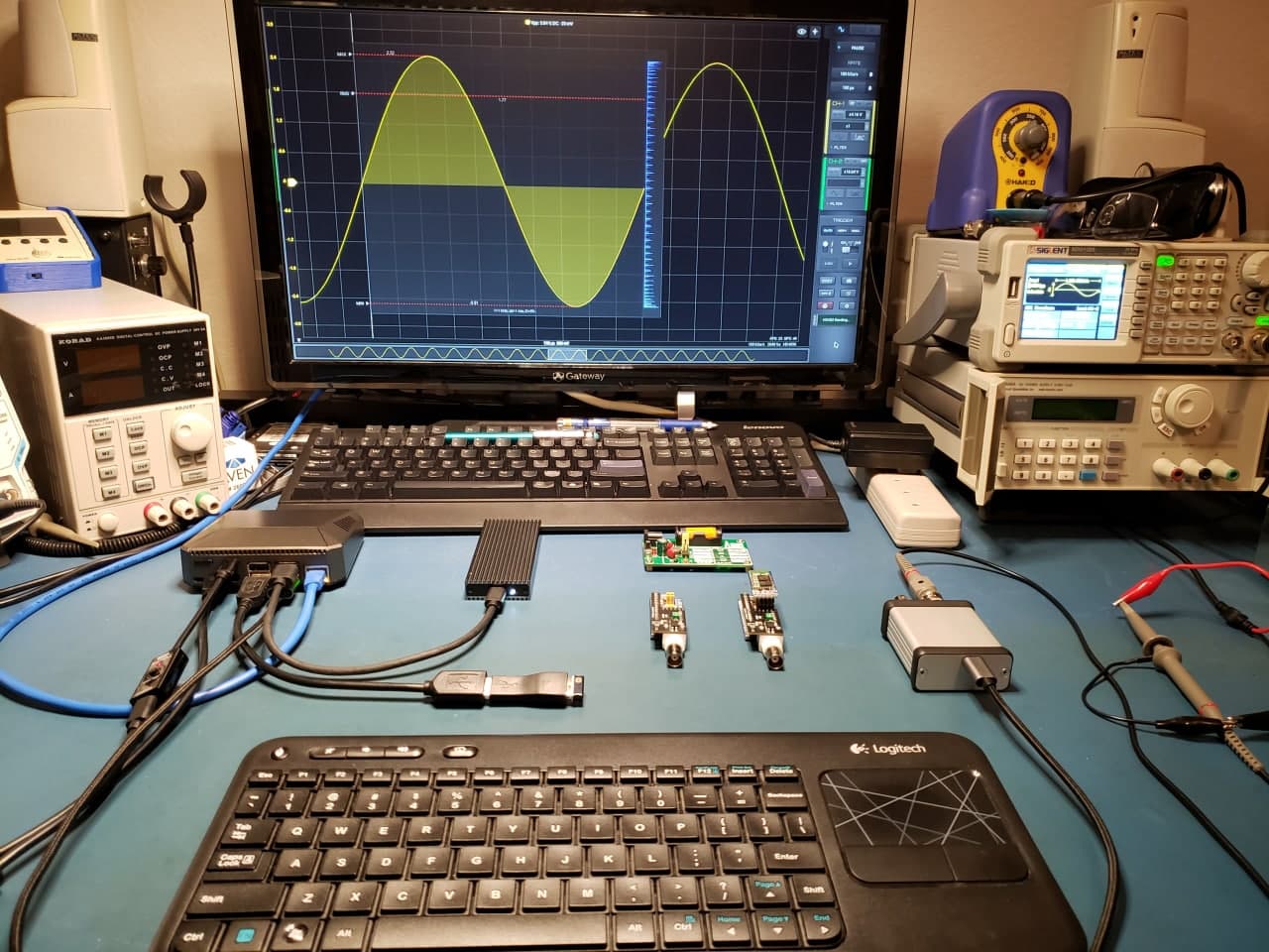
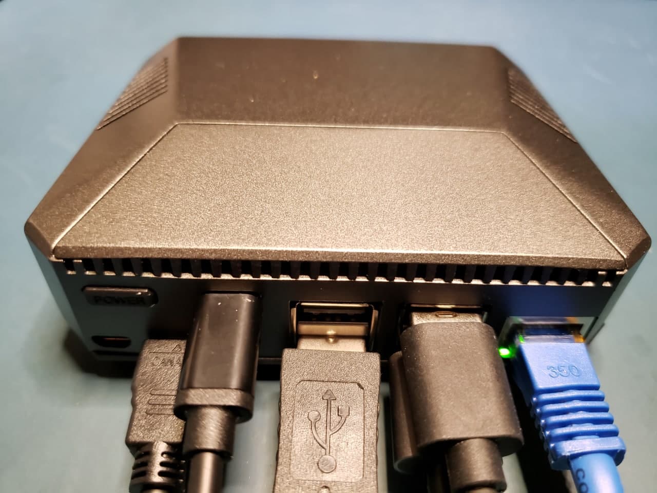
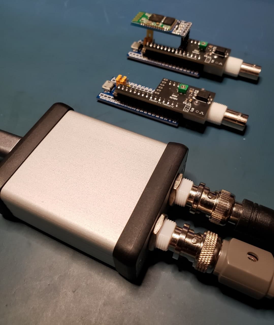
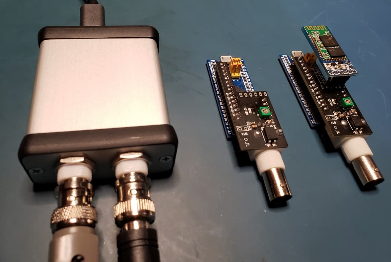
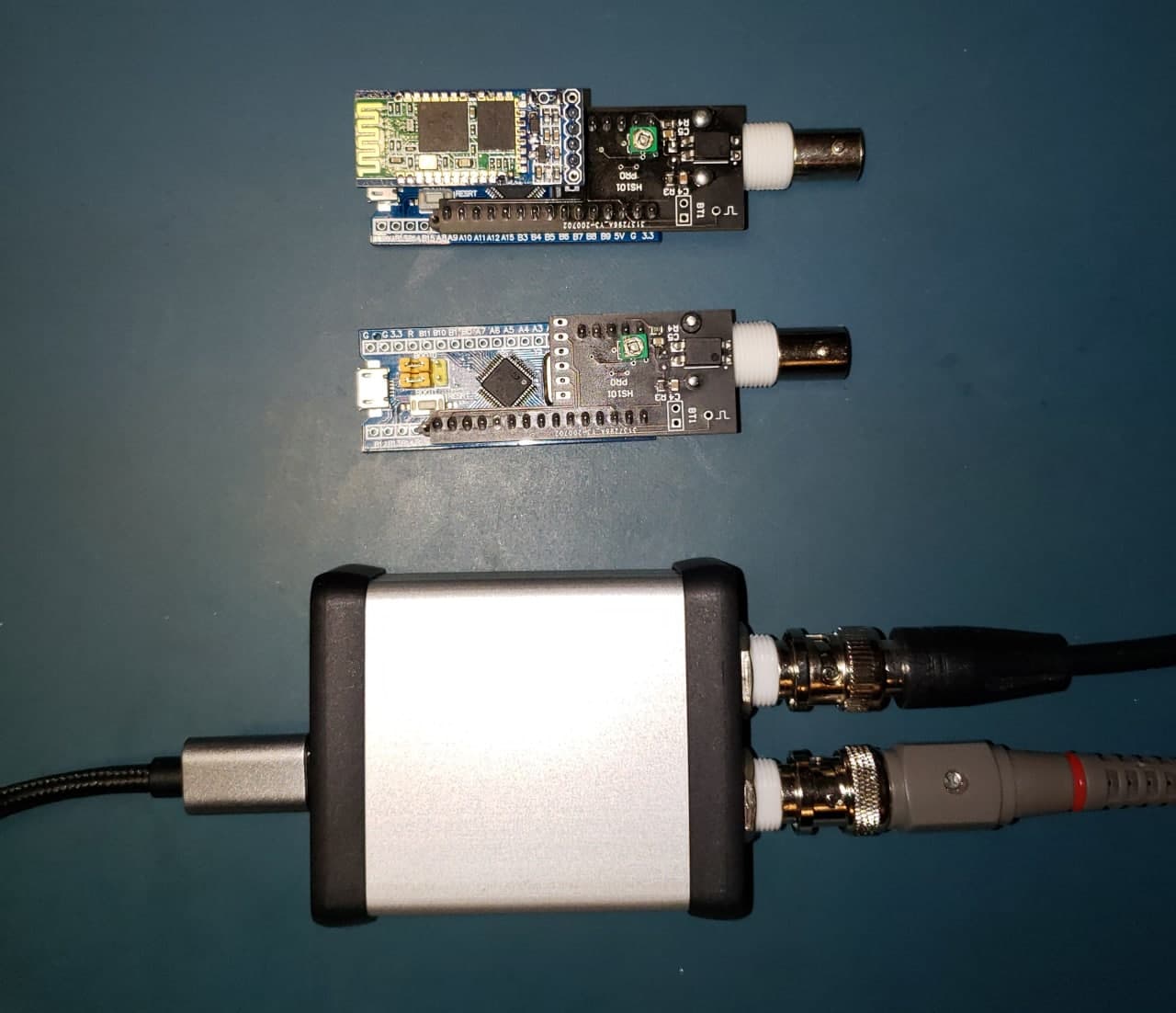
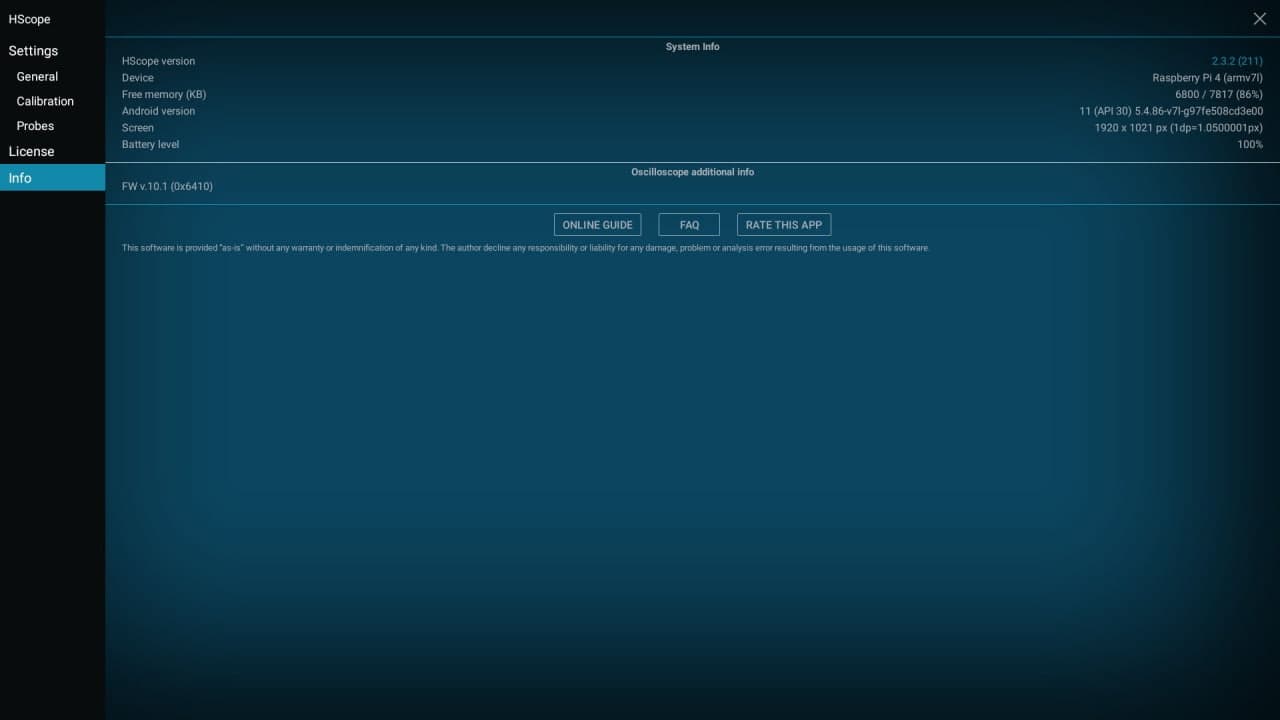
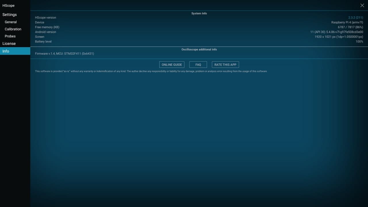
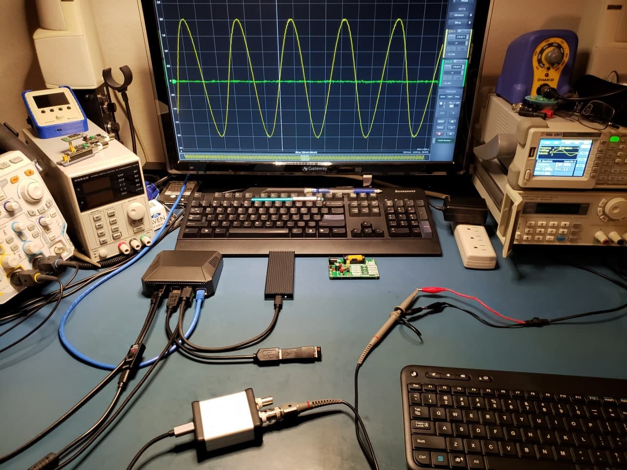
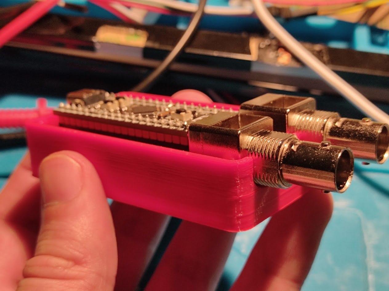
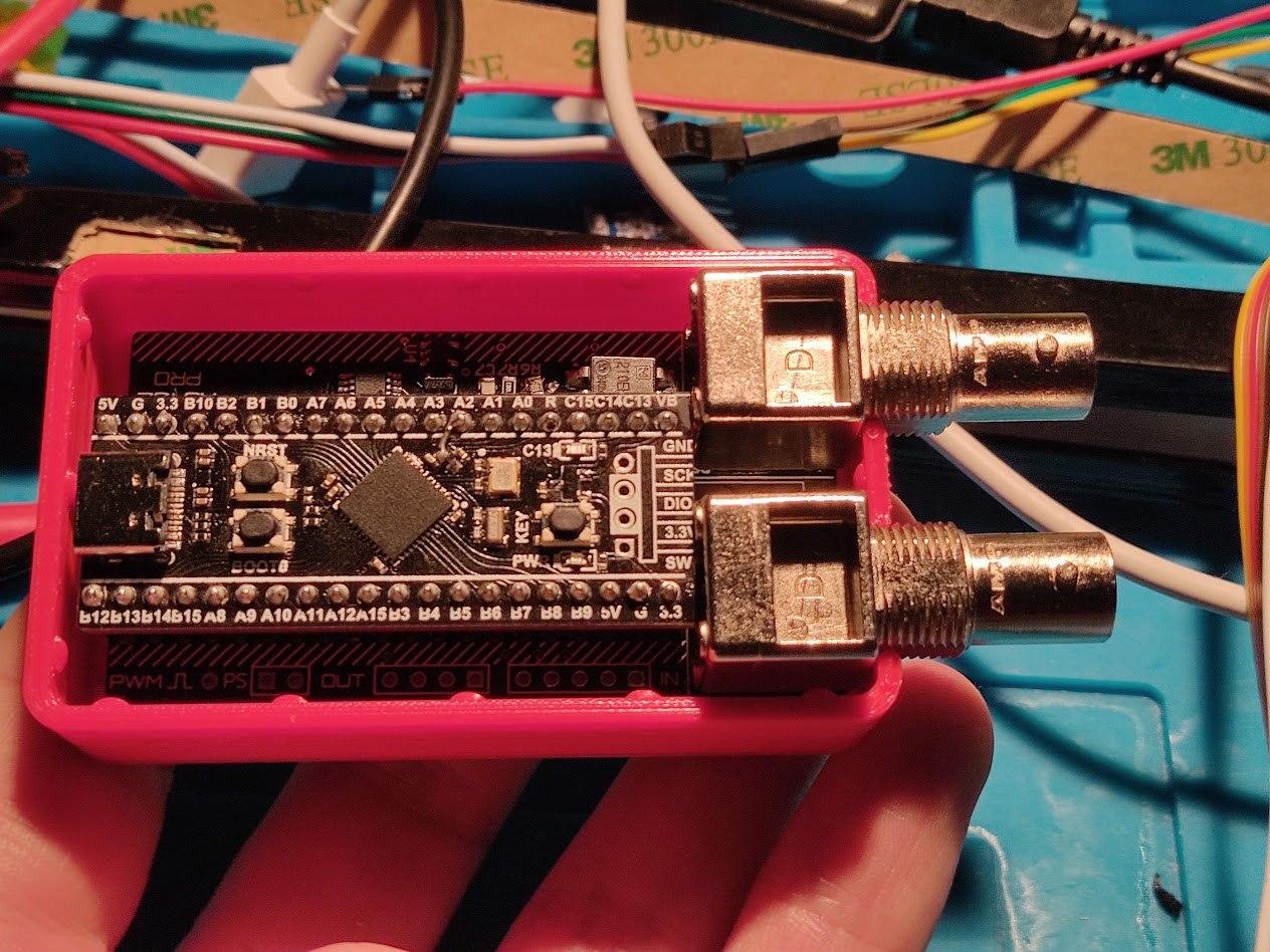
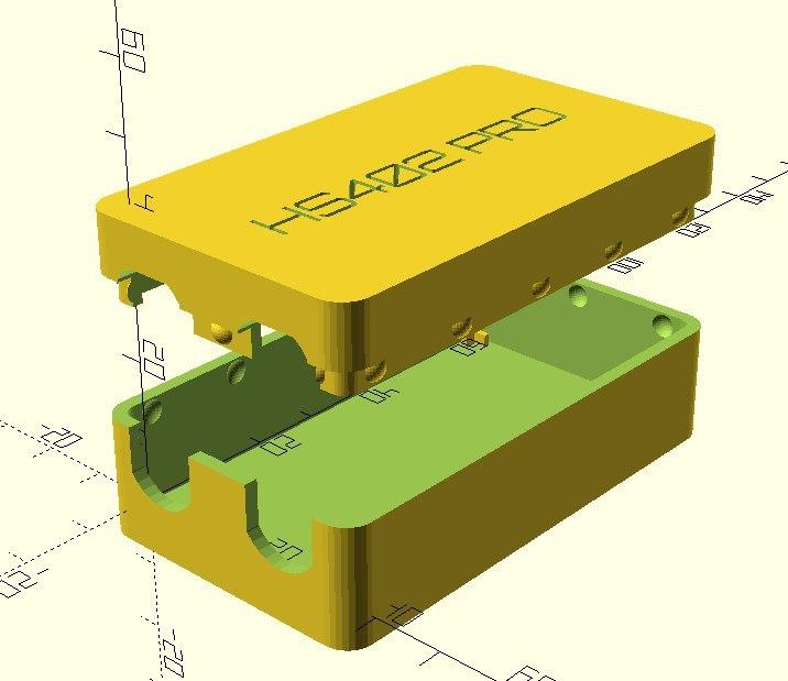
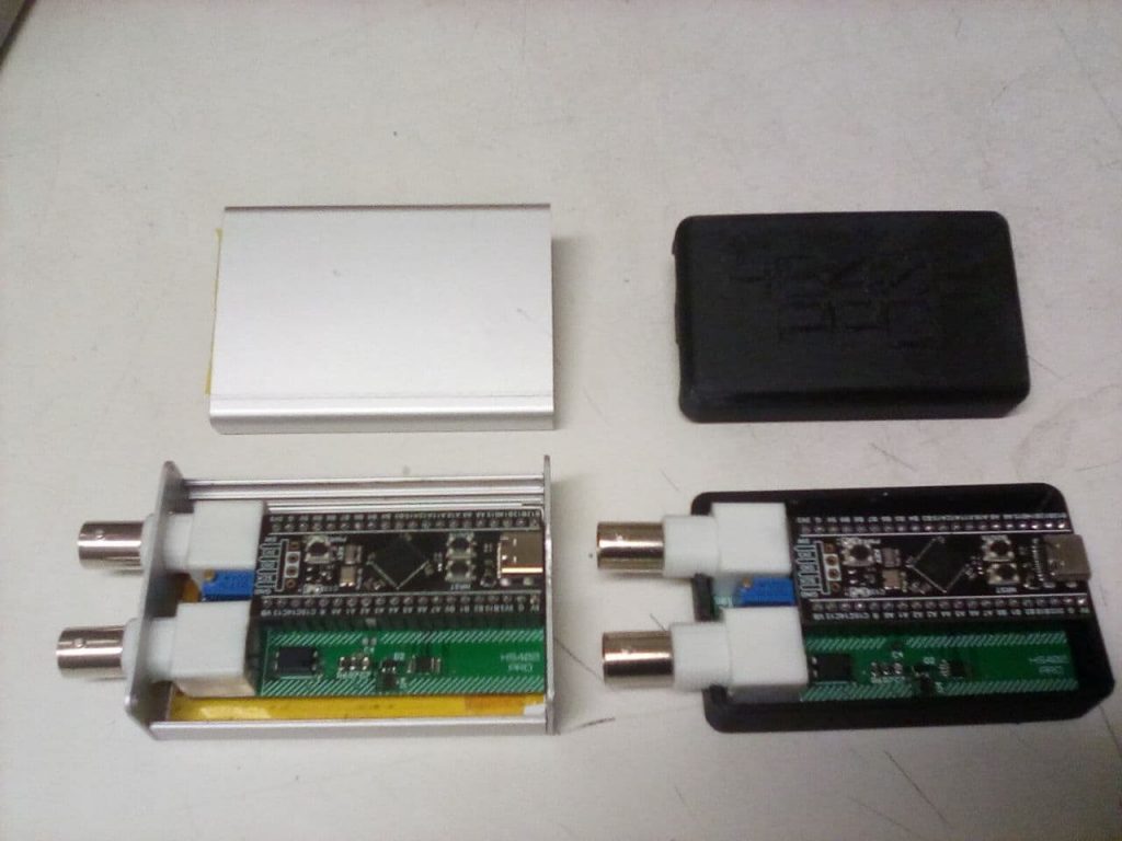
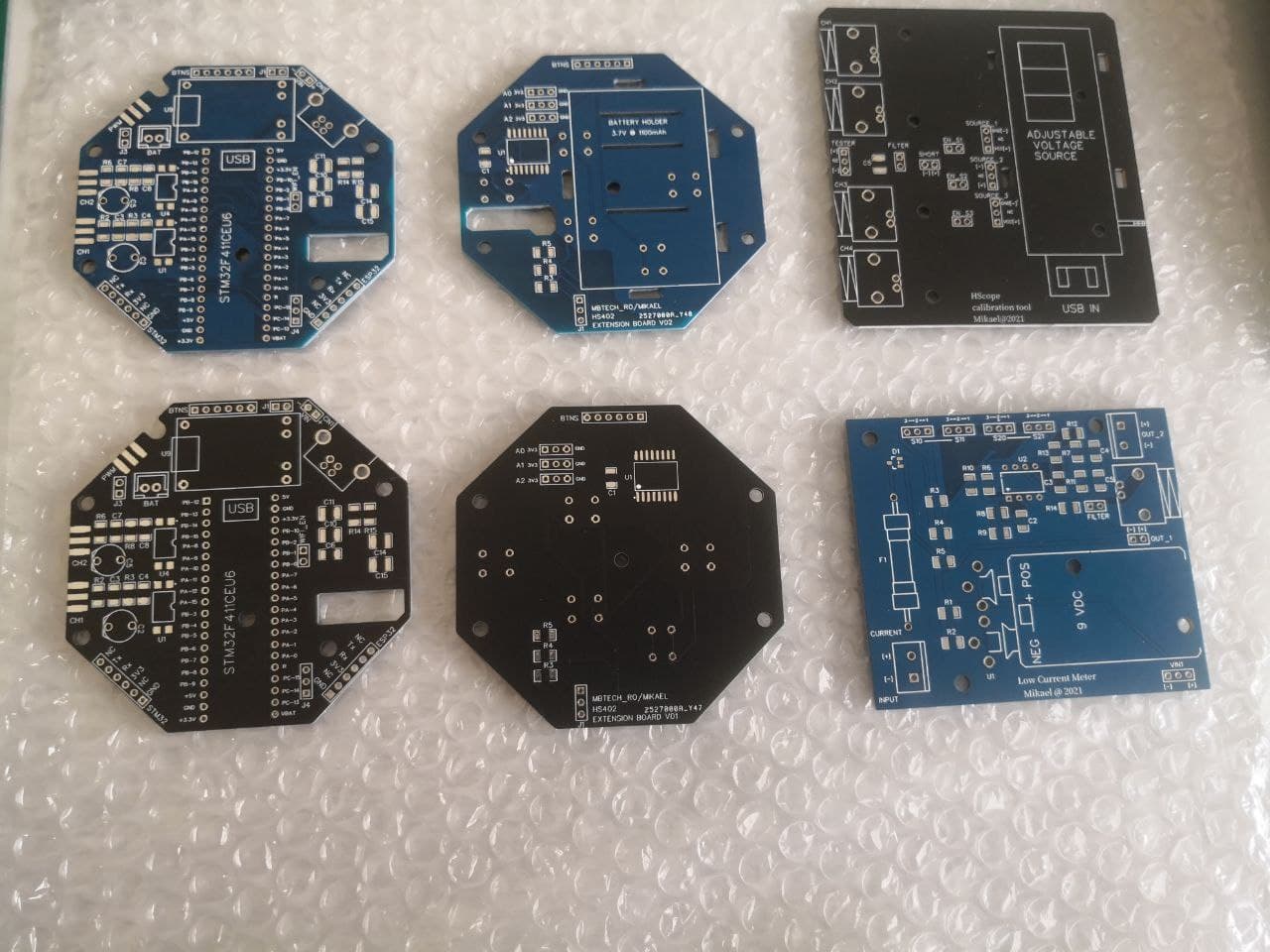
This setup has been made with a Raspberry Pi 4B inside a Argon ONE case. Attached are several pictures of a HS101 BLT, HS101 and HS402 all in action. The PI 4B has built in Bluetooth so it is possible to connect up the HS101 BLT.
Install Android 11 on Pi4
Here is the link to the Lineage OS 18.1 which is android version 11.
Here is link to google play store that will need to be installed. Dave found it easier to put the file on a USB drive and recommend putting this file on a separate USB drive for use later in the installation.
Tips
Install Android to microSD or to external SSD that uses USB. I tried a USB stick and android kept locking up.
Put the Google Play store file on a USB stick. I had significant issues trying to download the play store onto the Raspberry. Using a PC to download Google Play store and having it on the USB stick allowed installation per leepspvideo.
I tried separate USB mouse and keyboard. Mouse wouldn’t work. I had to use a logitech K400+ integrated touchpad and keyboard.
There is no pinch zooming. Its android thing. I mention this because you can double left click on the oscilloscope trace and HScope will zoom right in. But you have no way to zoom back out. What I learned to do was to toggle through “Auto/Norm/Single” selection. Then hit the play button. Then the trend zooms back out.
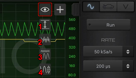
Align the waveform vertically keeping spacing among them.
Scale the second channel signal to fit the first channel signal (so to compare the shape).
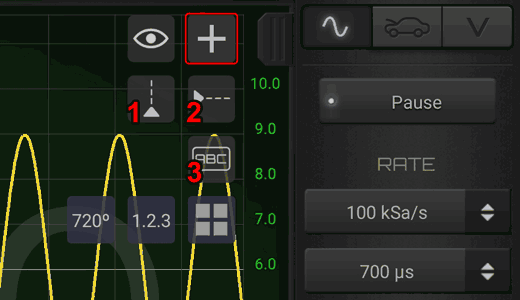
Press the “+” icon to activate the Supporting Tools.
Supporting Tools
Vertical Cursors: it show vertical cursor.
Horizontal Cursors: it create one horizontal cursor.
Annotation Tool: you can write labels on the graph and position them on the desired location.
Additional tools may be present according the additional modules installed (ie. Automotive Tools in the picture).
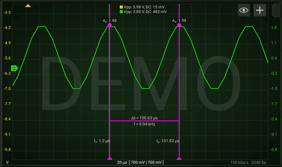
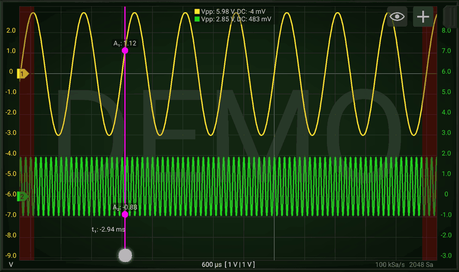
1. Vertical Cursors
Activating one vertical cursor allows you to measure amplitude of the signals at a certain point. By pressing 2 fingers on the bottom part of the graph you can enable 2 cursors and have relative measurements. (as time and frequency associated to the selected period).
2 Vertical Cursors and relative measurement
For removing the cursors just push them out of the screen (to the left or to the right), on the red area.
Vertical Cursor when selected shows red areas for deletion
HScope allows a maximum of 2 Vertical Cursors.
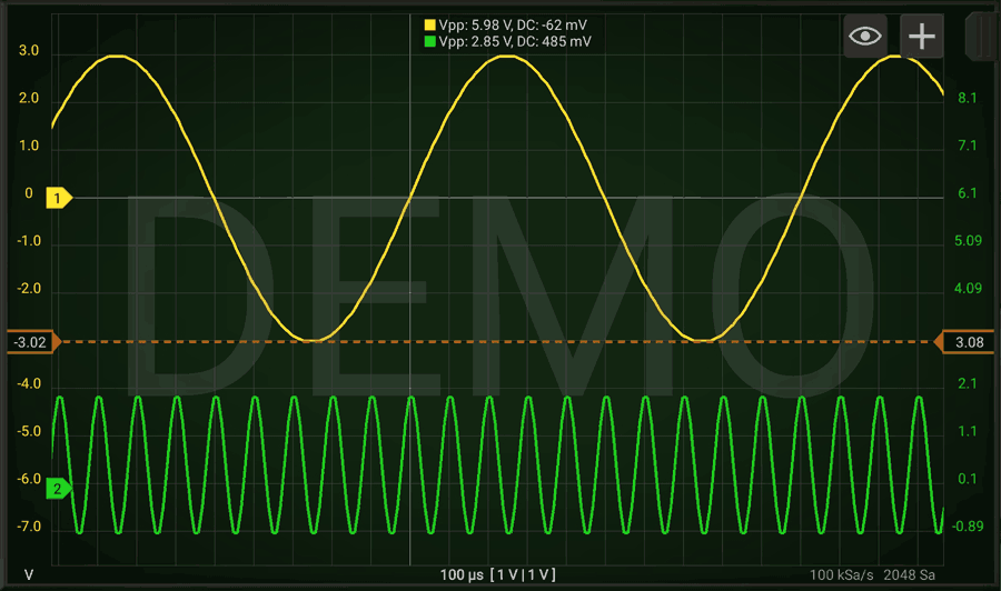
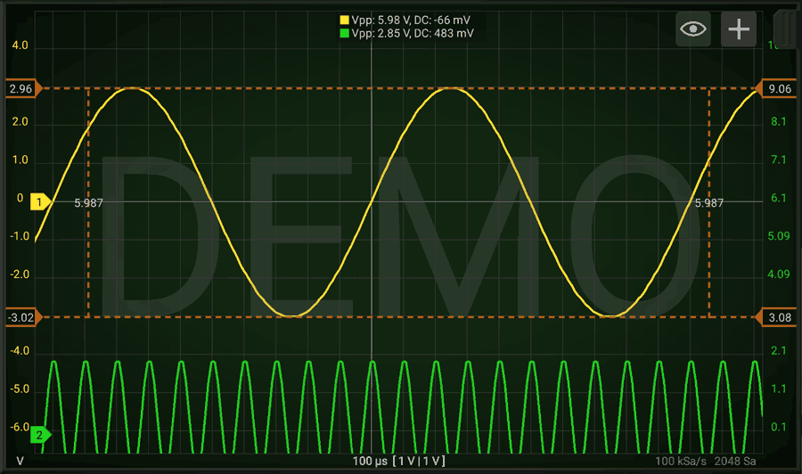
2. Horizontal Cursors
You can enable one or more Horizontal cursors. When you have 2 Horizontal cursors on the screen, you can see also the distance between the 2 cursors.
Horizontal cursors works as the Vertical ones.
Samples of Horizontal Cursors
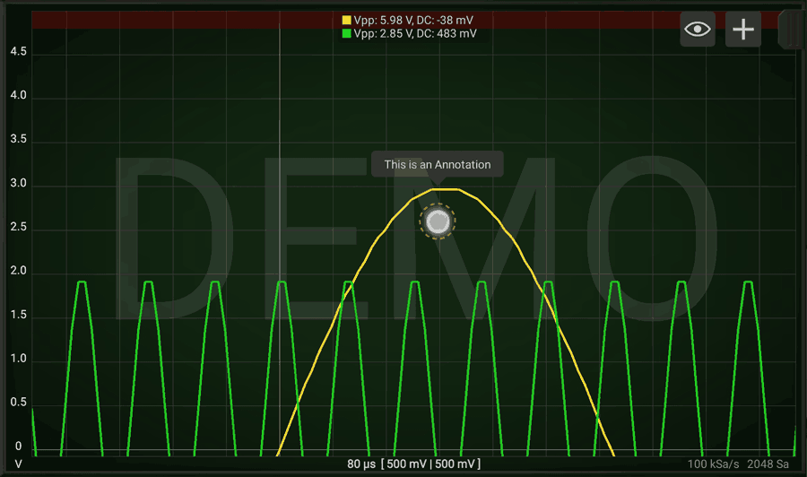
3. Annotation Tool
When you create a new Annotation you can set the text. Later you can change the location of the annotation but not its text. You can select an Annotation by clicking on it.
To delete an Annotation just move it behind the red bar.
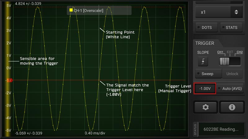
The Trigger allow you to see the signal stable on the screen since the Trigger set what is the starting point for drawing the signal. Even if the input signal can be periodic in some way, on each scan its position can be found translated since the acquisition time is random and it cannot be synchronous with the period of the input signal. The starting point for a signal can be identified with:
a Voltage Level (Trigger Level);
a tendency (or Slope) which means if the signal is passing the Voltage Level going up or down.
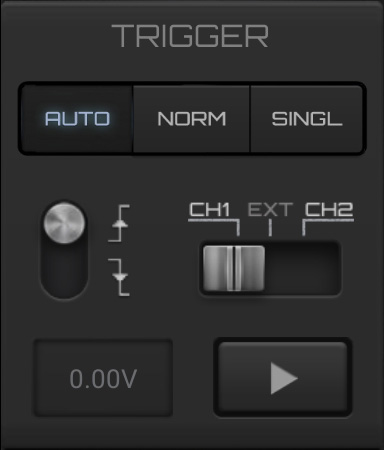
Trigger Panel
Once decided the kind of trigger (AUTO, NORMAL, SINGLE), you can set the SLOPE (arrow up or down) and the input Channel (only CH1 and CH2 are working and they are oscilloscope depending).
AUTO Trigger: set the Trigger Level as the middle level of the input voltage.
NORMAL Trigger: allow you to set the Voltage Level for the trigger. Every time the condition is met the signal is visualized on the screen.
SINGLE Trigger: as Normal Trigger but will show the signal just at the first occurrence of the condition, then it stops the acquisition. You can resume the acquisition by pressing the play button.
You can apply filters to each channel (button FILTER). Filtering operation may change the original signal in reversible or irreversible way. Irreversible filtering means that the operation modify the original signal in a way that later the original signal cannot be restored.
Type of Filtering
Description
Reversible
Invert (inversion)
It invert the input signal (the signal will be mirrored respect the 0 level)
Yes
Low Pass
The frequencies over the defined frequency will be attenuated.
No*
High Pass
The frequencies below the defined frequency will be attenuated.
No*
* In Automotive Module the filtering can be reversible until the waveform is not saved. After saving the filtered data will be saved and there is no way to reverse to the original waveform or change the filtering parameters.
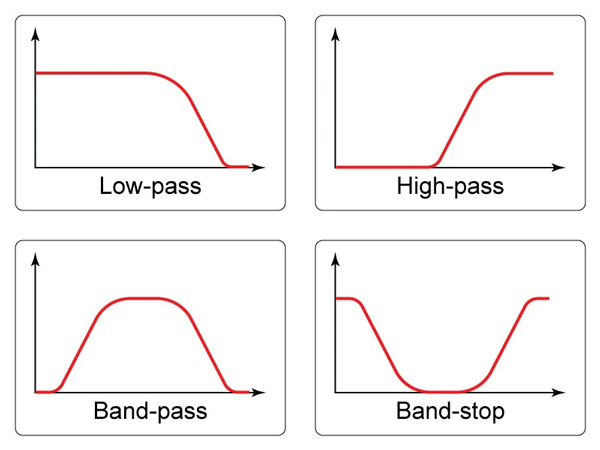
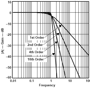
Filters Response in Frequency
You can set the cutoff frequency of the filter. In case of low-pass and high-pass filter you just set the one frequency, while in case of band-pass and band-stop filters you must set 2 frequecies, one of start and one of end. At the cutoff frequency the signal is attenuated of 70.7% of its amplitude and keep to be attenuated more an more according the graph above.
For example if you set a low-pass filter at 100Hz it means that you will see all the components of the signal up to around 100Hz. After 100Hz they will be progressively attenuated.
The inclination of the attenuation curve depends from the filter order. Higher is the order and more rapids is the curve.
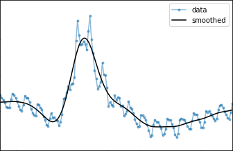
A typical usage of a low-pass filter is to filter out the noise from the signal of interest, a way to “clean” the waveform. Here an example of signal cleaning with a low-pass filter:
Differently from other oscilloscopes, in HScope you can set the voltage input range for each channel. The concept of Volts/division is just reported as information but it is not really practical since the signal can be zoomed and shifted on the screen and measured with absolute scales and relative cursors.
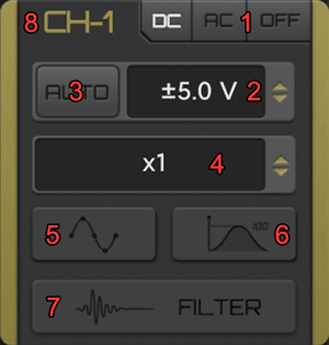
Channel Setting Panel
DC/AC/OFF Button: can switch the input coupling mode to DC, AC or switch off the channel.
Input Voltage Selector: it set the oscilloscope maximum input range.
AUTO Button: automatically switch the input voltage according the input signal.
Probe Selector: set the current hardware probe used by the oscilloscope on the channel.
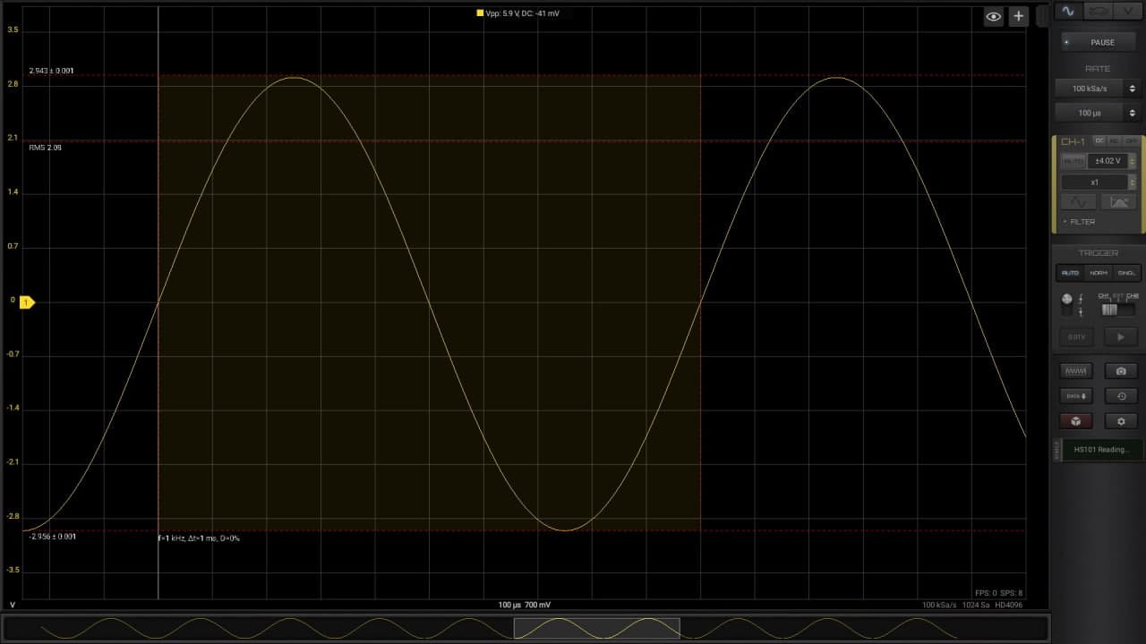
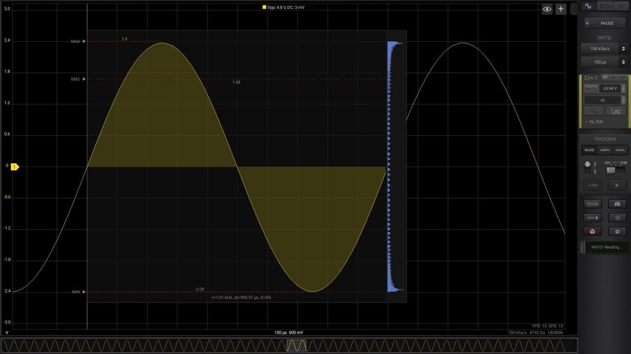
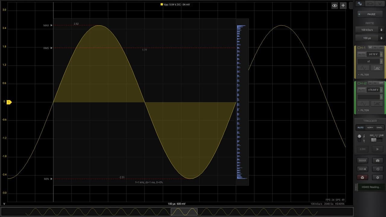
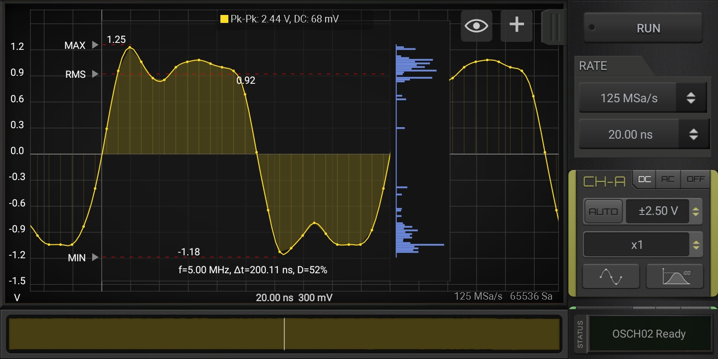
Samples Button: by enabling it you can see the actual samples by zooming in the signal on the screen.
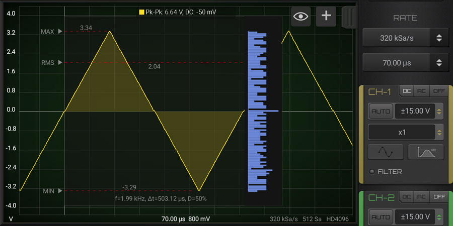
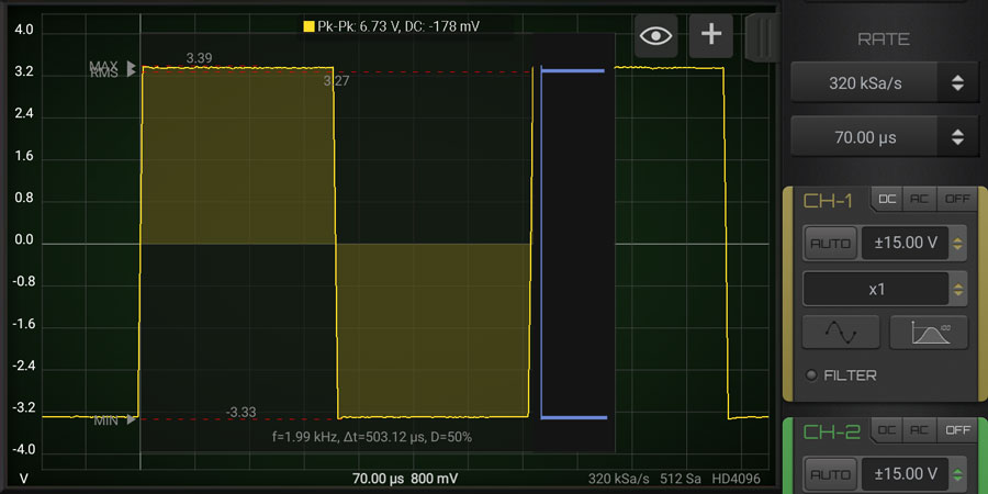
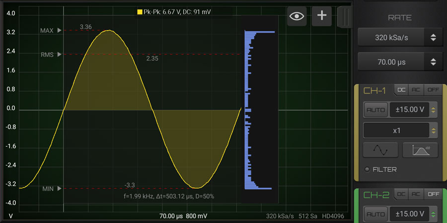
Statistics Button: it show the main statistics for periodic signals by showing the details of 1 period of the main frequency. HScope support 2 kind of statistics, press 1 time for the simple one, press another time for the Histogram, a last time to turn them off.
Filters: to enable filters on the channel (check the Filters section).
Channel Name: you can change the channel name by clicking here. The new name will be shown on the report and saved in the waveform file.
1. DC/AC/OFF Button
Selecting DC the signal goes to screen AS-IS (with AC and DC components), selecting AC the signal pass into a filter (that can be hardware or software according the device) so that on screen and in computation is considered just the AC component.
2. Input Voltage Selector
This value is oscilloscope depending and change according the actual calibration. To benefit of the highest vertical resolution it is suggested to use the lowest range which include the measured signal.
3. AUTO Button
Selecting the button AUTO the software automatically set the input voltage selector according to the signal. It is intended to be use only for time invariant signals (like a sine wave) otherwise the input range will be changed very time the input signal change. This function is limited just to high voltage ranges. Lower voltage selection should still come manually.
4. Probes Selector
This setting won’t affect the hardware settings but it will affect the final readings since the data will be computed according the probe settings.
IMPORTANT: Probe setting MUST reflect the probe hardware to avoid damage to the device or wrong readings. (ie: you can set x10 in HScope only if the hardware probe has x10 switch selected)
In case you need to measure stronger signals the Probe should have a switch that allow to attenuate the input signal. If you change the switch of your probe to the position x10, the input signal will be attenuated by a factor 10. This means that using the Oscilloscope range ±5V with a probe x10 you can see signals up to ±50V (50V / 10 = 5V). In visualization the App already calculate this scaling factor, so if you use a probe x10 just select in the Channel configurations the factor x10 and play with the voltage ranges (it will show you the possible range you can select).
On the market are available different kind of probes (also associated to different units like Ampere,…). You can add or download new probes in the Settings → Probes panel.
We use technologies like cookies to store and/or access device information. We do this to improve browsing experience and to show personalized ads. Consenting to these technologies will allow us to process data such as browsing behavior or unique IDs on this site. Not consenting or withdrawing consent, may adversely affect certain features and functions.
Functional
Always active
The technical storage or access is strictly necessary for the legitimate purpose of enabling the use of a specific service explicitly requested by the subscriber or user, or for the sole purpose of carrying out the transmission of a communication over an electronic communications network.
Preferences
The technical storage or access is necessary for the legitimate purpose of storing preferences that are not requested by the subscriber or user.
Statistics
The technical storage or access that is used exclusively for statistical purposes.The technical storage or access that is used exclusively for anonymous statistical purposes. Without a subpoena, voluntary compliance on the part of your Internet Service Provider, or additional records from a third party, information stored or retrieved for this purpose alone cannot usually be used to identify you.
Marketing
The technical storage or access is required to create user profiles to send advertising, or to track the user on a website or across several websites for similar marketing purposes.
 Guide
Guide